Week 7 - Simulation of a 1D Super-sonic nozzle flow simulation using Macormack Method

OBJECTIVE :

Stimulation of 1 - d supersonic nozzle both conservative and non -conservative form .

INTRODUCTION :

Super sonic nozzle : In simple terms a supersonic nozzle is basically a convergent-divergent nozzle . It is the capacity of the convergent-divergent nozzle to extract pressure/internal energy from a low-speed inlet flow completely and efficiently and generate supersonic exit velocities that make it a vital component of high-speed aerospace propulsion.

In this report we are studying how the flow parameters varry through out the length of the nozzle and the total no of time step , How the mass flow rate varies in the convergent - divergent nozzle , this is plotted down for both conservative and non - conservative forms . To start with the objective of the program we have to understand some basic concepts in fluid flow , the governing equations and solvers for pde .

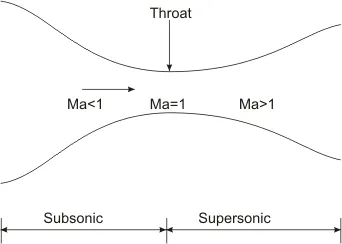
Figure 1 : super sonic nozzle

basically a supersonic convergent divergent nozzle acclerates the speed of the air flowing out of the nozzle , from the figure at the inlet the mach is 1 and at the outlet the mach is greater 1 , the above figure is the sample pictorial refrence of our current problem . so from the figure we can conclude on some results which are

`M = V/a`

a = speed of sound

1. so , `V_(out) > (V_(i nl et))`
2. we know that the pressure is inversely propotional to velocity , so `P_(i nl et)>P_(outl et)` .
3. we know that p = `rho *r* t` , so if the pressure at the outlet decrease , the density and the temperature also decreases at the outlet also decreases .

so basically we are going to study the change in this parameters Mach no , density , pressure, velocity and temperature with respect to time through out the nozzle . The flow parameters at th the throat are known as critical parameters , or chocked condition , In this report we will also see how the flow parameters behave in the chocked as a function of time . The cross- sectional area of the nozzle is defined as a . Here we make an assumption that the flow properties varry only along the x- axis , such flow is defined as quassi-one dimensional flow. The governing equations for the quasi one dimensional flow ( conservative and Non - conservative forms are as shown : )

Continuity Equation :

`rho_1*v_1*a_1 = rho_2 *a_2*v_2`.........(1)

`(partialrho*a)/(partialt) +(partialrho*a*v)/(partialt) = 0`........(2)

In this report we are not looking at the derrivations of governing equation , the final equations and the derrivations are taken from " computational fluid dynamics book" jd . Anderson . The governing equations are as follows :

continuity : `(partial(rhoA))/(partialt) + rhoA(partialv)/(partialx) + rhov(partialA)/(partialx) + VA(partialrho)/(partialx) = 0`.............(3)

Momentum : `rho(partialV)/(partialt) + rhov( partialv)/dx = -Rrho(partialT)/(partialx) -RT(partialrho)/(partialx)`.............(4)

Energy : `rhoc_v(partialT)/(partialt) + rhoVc_v(partialT)/(partialx) = - rhoRT[(partialV)/(partialx) + v(partial( ln A))/(partialx)]` ....................(5)

Equation 3 - 5 are written in terms of dimensional variables and its a added advantage but for nozzle flow the eqyations are used in the form of non dimensional variables which are as follows :

`T' = T / T_0`

`rho' = rho/rho_o`

`x' = x/l`

`v' = v/a_0`

`t' = t/(L/a_0)`

`A' = A / A*`

`a_0 = sqrt ( gammart)`

Now substitute the non-dimensionless in the quantity in the equations 3 , 4 and 5 and we get the equations in the non-conservative form for the computational methods as :

continuity : `(partialrho')/dt = -rho'(partialv')/(partialx) -rho'v'(partial(ln A'))/(partialx')- v'(partialrho')/(partialx')`...................(6)

Momentum : `(partialV')/(partialt') = -V'*(partialV')/(partialx') - 1/gamma * ((partialT')/(partialx') + (T')/(pho')*(partialrho')/(partialx'))`......................(7)

Energy :`(partialT')/(partialt') = -V'(partialT')/(partialx') - (gamma-1)T'[(partialV')/(partialx') + V'*(partial(lnA'))/(partialx')]`...............................(8)

The equations from 6 to 8 is used to compute the stimulation of 1-d supersonic nozzle .

Conservative form :

............................................(9)

..............................(10)

....................................(11)

eq 9 to 11 represent the continuity, Momentum and Energy equation in the conservative form which the equations for the stimulation of 1-d supersonic Nozzle is formulated using the macromaks method using the predictor and corrector steps.

CODE :

close all 
clear all
clc 
l = 3 ;
n = 31;
x = linspace(0,l,n);
dx = x(2)-x(1);
nt = 1400 ;
throat = 16 ;
C = 0.5 ;
gama = 1.4;
tic 
[a,dt,nt_grid,mass_flow,mach_no,pressure,temp_t_0,rho_t_0,mass_flow_throat,pressure_t,temp_t_0_throat,mach_no_throat,v_t_0_throat,rho_t_0_throat] = non_conservative_form(l,n,x,dx,nt,throat,gama,C);
t_non_conservative = toc 
tic 
[nt_grid_c,mass_flow_c,mass_flow_c_t,mach_no_c_t,mach_no_c,rho_c,rho_c_t,pressure_c_t, pressure_c,temp_c,temp_c_t,v_c,v_c_t] = conservative_form_final(x,n,dx,gama,nt,a,C,throat);
t_conservative = toc 
% grid independece test 
% % calculating the values at throat 
terms = {'Non-Dimensional Density';'Non-Dimensional Temperature';'Non-dimensional pressure';'Mach Number'};
exact_solution = [ 0.634 ; 0.8333 ; 0.528 ; 1];
non_conservative_terms = [rho_t_0(throat);temp_t_0(throat);pressure(throat);mach_no(throat)];
conservative_terms = [rho_c(throat);temp_c(throat);pressure_c(throat);mach_no_c(throat)];
table(terms, exact_solution,non_conservative_terms,conservative_terms)
figure(3)
plot(x,mass_flow,'r','linewidth',2)
hold on
plot(x,mass_flow_c,'b','linewidth',2)
title('comparission of Non-dimensional mass flow rates')
xlabel('x/l')
ylabel('Non-dimensional mass flow rate ')
grid on 
figure(4)
subplot(4,1,1)
plot(x,mach_no,'r','linewidth',2)
title('Variation of different flow parameters : Non conservative form ','Fontsize',20,'Fontweight','bold','color','black')
xlabel('x-axis')
ylabel('Mach no')
subplot(4,1,2)
plot(x,rho_t_0,'b','linewidth',2)
xlabel('x-axis')
ylabel('Density ratio')
subplot(4,1,3)
plot(x,pressure,'g','linewidth',2)
xlabel('x-axis')
ylabel(' Pressure ratio')
subplot(4,1,4)
plot(x,temp_t_0,'black','linewidth',2)
xlabel('x-axis')
ylabel('Temperature ratio')

figure(5)
subplot(4,1,1)
plot(nt_grid,mach_no_throat,'r','linewidth',2)
title('Variation of different flow parameters at the ''Throat section'' of the nozzle: Non conservative form','Fontsize',20,'Fontweight','bold','color','black')
xlabel('No of time step')
ylabel('Mach no')
subplot(4,1,2)
plot(nt_grid,rho_t_0_throat,'b','linewidth',2)
xlabel('No of Time-step')
ylabel('Density ')
subplot(4,1,3)
plot(nt_grid,pressure_t,'g','linewidth',2)
xlabel('No of Time-step')
ylabel(' Pressure ')
subplot(4,1,4)
plot(nt_grid,temp_t_0_throat,'black','linewidth',2)
xlabel('No of Time-step')
ylabel('Temperature')

figure(6)
subplot(4,1,1)
plot(x,mach_no_c,'r','linewidth',2)
title('Variation of different flow parameters :  conservative form ','Fontsize',20,'Fontweight','bold','color','black')
xlabel('x-axis')
ylabel('Mach no')
subplot(4,1,2)
plot(x,rho_c,'b','linewidth',2)
xlabel('x-axis')
ylabel('Density ratio')
subplot(4,1,3)
plot(x,pressure_c,'g','linewidth',2)
xlabel('x-axis')
ylabel(' Pressure ratio')
subplot(4,1,4)
plot(x,temp_c,'black','linewidth',2)
xlabel('x-axis')
ylabel('Temperature ratio')

figure(7)

subplot(4,1,1)
plot(nt_grid_c,mach_no_c_t,'r','linewidth',2)
title('Variation of different flow parameters at the ''Throat section'' of the nozzle : conservative form','Fontsize',20,'Fontweight','bold','color','black')
xlabel('No of time step')
ylabel('Mach no')
subplot(4,1,2)
plot(nt_grid_c,rho_c_t,'b','linewidth',2)
xlabel('No of Time-step')
ylabel('Density ')
subplot(4,1,3)
plot(nt_grid_c,pressure_c_t,'g','linewidth',2)
xlabel('No of Time-step')
ylabel(' Pressure ')
subplot(4,1,4)
plot(nt_grid_c,temp_c_t,'black','linewidth',2)
xlabel('No of Time-step')
ylabel('Temperature')

Fig 2 : Main program code for the stimulation of 1-d super-sonic nozzle for both conservative and Non-conservative form

function[nt_grid_c,mass_flow_c,mass_flow_c_t,mach_no_c_t,mach_no_c,rho_c,rho_c_t,pressure_c_t, pressure_c,temp_c,temp_c_t,v_c,v_c_t] = conservative_form_final(x,n,dx,gama,nt,a,c,throat);
% Initializing the solution 

for j = 1: n
    if (x(j)>=0 && x(j)<=0.5)
        rho_c(j) = 1;
        temp_c(j) = 1 ;
    elseif (x(j)>=0.5 && x(j)<=1.5)
        rho_c(j) = 1 - (0.366*(x(j)-0.5));
        temp_c(j) = 1 - (0.167*(x(j)-0.5)) ;
    elseif (x(j)>=1.5 && x(j)<=3.5)
        rho_c(j) = 0.634 - (0.3879*(x(j)-1.5));
        temp_c(j) = 0.833 - (0.3507*(x(j)-1.5)) ; 
    end
end

% initial conditions
v_c = 0.59./(rho_c.*a);
mass_flow_c = rho_c.*a.*v_c ;
mass_flow_analytical = 0.579*ones(n);
initial_mass_flow_c = rho_c.*v_c.*a ;
u_1 = rho_c.*a;
u_2 = u_1.*v_c ;
u_3 = u_1.*((temp_c/(gama -1))+(gama/2).*(v_c.^2));
nt_grid_c = linspace(1,nt,nt);
% dt = 0.002 ;  % min(c.*(dx./((temp.^0.5)+v))) ; % Time step 
% time loop 
for k = 1: nt 
    Dt = temp_c.^0.5 ;
    dt = min(c.*(dx./((temp_c.^0.5)+v_c)));
    u1_old = u_1 ;
    u2_old = u_2 ;
    u3_old = u_3 ;
    % Flux vector 
    f1 = u_2 ;
    f2_1 = (u_2.^2)./u_1 ;
    f2_2 = u_3 - ((gama/2)*f2_1);
    f2 = f2_1 + ((gama-1)/gama)*f2_2 ;
    f3_1 =( u_2.*u_3)./u_1 ;
    f3_2 = ( u_2.^3)./(u_1.^2) ;
    f3 = gama.*f3_1 - ((gama*(gama-1))/2).*f3_2 ;
    % Predictor step 
    for i = 2: n-1 
        j2_p(i) = ( 1/ gama)*(rho_c(i)*temp_c(i))*((a(i+1)-a(i))/dx);
        du1_dt_p(i) = -(f1(i+1)-f1(i))/dx ;
        du2_dt_p(i) = (-(f2(i+1)-f2(i))/dx) + j2_p(i) ;
        du3_dt_p(i) = -(f3(i+1)-f3(i))/dx ;
        % solution update 
        u_1(i) = u_1(i) + du1_dt_p(i)*dt ;
        u_2(i) = u_2(i) + du2_dt_p(i)*dt ;
        u_3(i) = u_3(i) + du3_dt_p(i)*dt ;
    end
    % updating the values 
    rho_c = u_1./a ;
    v_c = u_2./u_1 ;
    temp_c = (gama-1)*((u_3./u_1)-(gama/2)*(v_c.^2));
    f1 = u_2 ;
    f2_1 = (u_2.^2)./u_1 ;
    f2_2 = u_3 - ((gama/2)*f2_1);
    f2 = f2_1 + ((gama-1)/gama)*f2_2 ;
    f3_1 = (u_2.*u_3)./u_1 ;
    f3_2 = (u_2.^3)./(u_1.^2);
    f3 = gama.*f3_1 -((gama*(gama-1))/2).*f3_2 ;
    
    % corrector step 
    
     for i = 2: n-1 
         j2_c(i) = ( 1/ gama)*(rho_c(i)*temp_c(i))*((a(i)-a(i-1))/dx);
         du1_dt_c(i) = -(f1(i)-f1(i-1))/dx ;
         du2_dt_c(i) = (-(f2(i)-f2(i-1))/dx) + j2_c(i) ;
         du3_dt_c(i) = -(f3(i)-f3(i-1))/dx ;
     end
     % Average values 
     du1_dt_avg = 0.5 * (du1_dt_p + du1_dt_c);
     du2_dt_avg = 0.5 * (du2_dt_p + du2_dt_c);
     du3_dt_avg = 0.5 * (du3_dt_p + du3_dt_c);
     for z = 2:n-1 
         u_1(z) = u1_old(z) + du1_dt_avg(z)*dt ;
         u_2(z) = u2_old(z) + du2_dt_avg(z)*dt ;
         u_3(z) = u3_old(z) + du3_dt_avg(z)*dt ;
     end

Fig 3 : Function program for stimulation of 1-d supersonic nozzle (conservative form )

% 1 -D super sonic nozzle stimulation 
% Function program with Non-conservative form 

% INITIAL CONDITIONS AT TIME ( T = 0)
% DENSITY , TEMPERATURE AND VELOCITY
function[a,dt,nt_grid,mass_flow,mach_no,pressure,temp_t_0,rho_t_0,mass_flow_throat,pressure_t,temp_t_0_throat,mach_no_throat,v_t_0_throat,rho_t_0_throat] = non_conservative_form(l,n,x,dx,nt,throat,gama,C)
rho_t_0 = 1- 0.314*x ;
temp_t_0 = 1- 0.2314*x ; 
v_t_0    = (0.1 + 1.09*x).*(temp_t_0.^(0.5));
a = 1+ (2.2*(x-1.5).^2);
mass_flow_analytical = 0.579*ones(n);
initial_mass_flow = rho_t_0.*v_t_0.*a ;
nt_grid = linspace(1,nt,nt);





% time step
% dt(i)= C.*(dx./((temp(i)).^0.5+v(i)));
dt= min(C*(dx./(temp_t_0.^0.5+v_t_0)));
% Time loop 
for k = 1: nt 
   % keeping a copy of values 
   rho_old = rho_t_0 ;
   temp_old = temp_t_0 ;
   v_old = v_t_0 ;
  
   % Macromack maethod 
   for j = 2:n-1 % Loop creation for internal grid points 
       dvdx =(v_t_0(j+1)-v_t_0(j))/dx ;
       dlog_a_dx = (log(a(j+1))-log(a(j)))/dx ;
       drho_dx = (rho_t_0(j+1)- rho_t_0(j))/dx ;
       dtemp_dx = ( temp_t_0(j+1)-temp_t_0(j))/dx ;
       
       % continuity equation 
       drho_dt_p(j) = -(rho_t_0(j)*dvdx)-(rho_t_0(j)*v_t_0(j)*dlog_a_dx)-(v_t_0(j)*drho_dx);
       % Momentum equation 
       dvdt_p(j) = -v_t_0(j)*dvdx - (1/gama)*(dtemp_dx + (temp_t_0(j)/rho_t_0(j))*(drho_dx));
       % Energy equation : 
       dtemp_dt_p(j) = - v_t_0(j)*dtemp_dx - (gama-1)*temp_t_0(j)*(dvdx + (v_t_0(j)*dlog_a_dx));
       
       % solution update at time step t + dt 
       rho_t_0(j) = rho_t_0(j)+ drho_dt_p(j)*dt ;
       v_t_0(j)   = v_t_0(j) + dvdt_p(j)*dt ;
       temp_t_0(j)   = temp_t_0(j) + dtemp_dt_p(j)*dt ; 
   end
   % corrector step 
    for j = 2:n-1 % Loop creation for internal grid points 
       dvdx =(v_t_0(j)-v_t_0(j-1))/dx ;
       dlog_a_dx = (log(a(j))-log(a(j-1)))/dx ;
       drho_dx = (rho_t_0(j)- rho_t_0(j-1))/dx ;
       dtemp_dx = ( temp_t_0(j)-temp_t_0(j-1))/dx ;
       
       % continuity equation 
       drho_dt_c(j) = -(rho_t_0(j)*dvdx)-(rho_t_0(j)*v_t_0(j)*dlog_a_dx)-(v_t_0(j)*drho_dx);
       % Momentum equation 
       dvdt_c(j) = -v_t_0(j)*dvdx - (1/gama)*(dtemp_dx + (temp_t_0(j)/rho_t_0(j))*(drho_dx));
       % Energy equation : 
       dtemp_dt_c(j) = - v_t_0(j)*dtemp_dx - (gama-1)*temp_t_0(j)*(dvdx + (v_t_0(j)*dlog_a_dx));
       
       
    end
   % Airthmetic mean final step 
   drho_dt_avg = 0.5 *(drho_dt_p + drho_dt_c);
   dvdt_avg = 0.5 * ( dvdt_p + dvdt_c ) ;
   dtemp_dt_avg = 0.5 * ( dtemp_dt_p + dtemp_dt_c) ;
   
   for i = 2: n-1 
        rho_t_0(i) = rho_old(i)+ drho_dt_avg(i)*dt ;
        v_t_0(i)   = v_old(i) + dvdt_avg(i)*dt ;
        temp_t_0(i)  = temp_old(i) + dtemp_dt_avg(i)*dt ; 
   end
   
   % boundry counditions 
   v_t_0(1) = (2*v_t_0(2))-v_t_0(3) ; % Inlet 
   % outlet
   v_t_0(n) = (2*v_t_0(n-1))-v_t_0(n-2) ;
   rho_t_0(n) = (2*rho_t_0(n-1))- rho_t_0(n-2) ;
   temp_t_0(n) = (2* temp_t_0(n-1))- temp_t_0(n-2);
   % calculating the mass flow rate 
   mass_flow = rho_t_0.* v_t_0.* a ;
   mach_no = v_t_0./(temp_t_0.^0.5);
   pressure = rho_t_0.*temp_t_0 ;
   
   % Defining the flow parameters at the throat 
   pressure_t(k) = pressure(throat);
   v_t_0_throat(k) = v_t_0(throat) ;
   rho_t_0_throat(k)  = rho_t_0(throat) ;
   temp_t_0_throat(k) =   temp_t_0(throat);
   mass_flow_throat(k) = mass_flow(throat);
   mach_no_throat(k) = mach_no(throat) ;
   
   % comparission of the mass flow rates at the different times 
   figure(1) 
   hold on 
   if k ==50
       plot(x,mass_flow,'r','linewidth',2)
   else if k ==100
       plot(x,mass_flow,'g','linewidth',2)
   else if k ==200 
       plot(x,mass_flow,'b','linewidth',2)
   else if k ==700
       plot(x,mass_flow,'y','linewidth',2)
       hold on 
       plot(x,mass_flow_analytical,'black','linewidth',2)
       hold on 
       plot(x,initial_mass_flow,'--','linewidth',2)
       
       title ('variation of mass flow distribution in non conservation form');
       legend('50 delta t','100 delta t','200 delta t','700 delta t','analytical solution','initial massflow');
       xlabel('Non- dimensional length of the nozzle');
       ylabel(' Mass flow rate')
       grid on
       pause(0.03)
       end
       end
       end
   end
end
end

Fig 4 : Function program for stimulation of 1-d supersonic nozzle ( Non-conservative form )

Results and output :

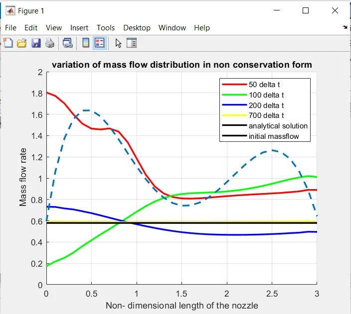
Fig 4 : variation of mass flow non conservative form

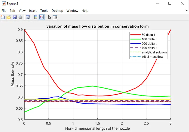
Figure 5 : Variation of Mass flow conservative form

Figure 6 : Comparission of mass flow rates betwwen conservative and non conservative forms

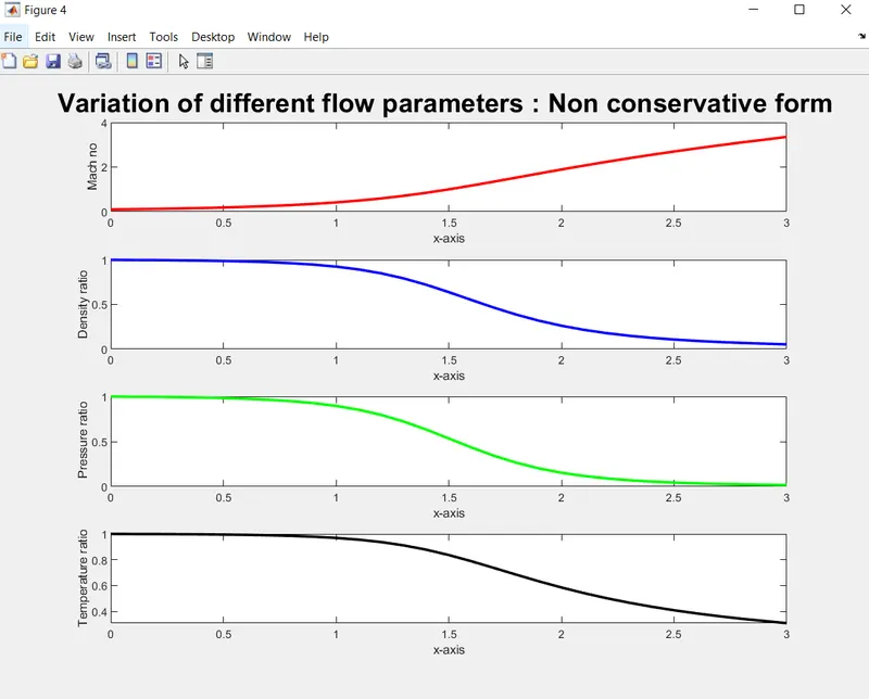
Figure 7 : Variation of Mass flow rates in Non conservative form

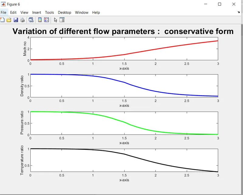
Figure 8 : Variation of mass flow rate in conservative form

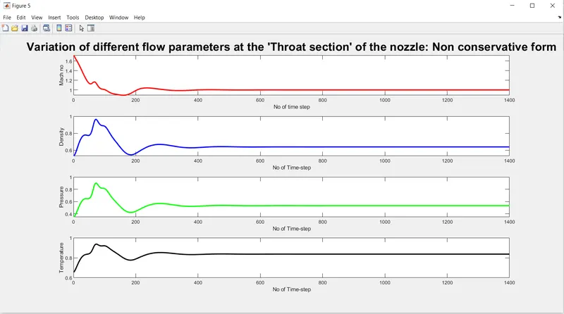
Figure 9 : Variation of mass flow rate parameters in the throat section ((Non conservative form)

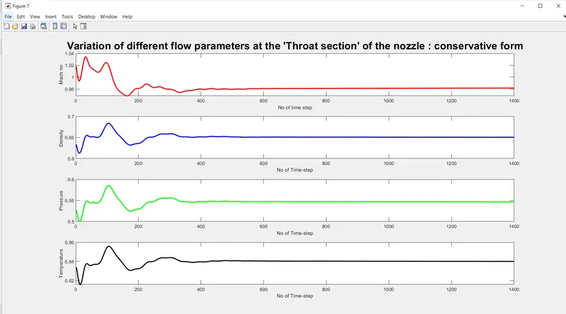
Figure 10 : Variation of mass flow rate parameters in the throat section (conservative form)

t_non_conservative =

    8.7652


t_conservative =

    5.6127


ans =

  4×4 table

                 terms                 exact_solution    non_conservative_terms    conservative_terms
    _______________________________    ______________    ______________________    __________________

    {'Non-Dimensional Density'    }         0.634               0.63866                 0.65039      
    {'Non-Dimensional Temperature'}        0.8333               0.83645                 0.84005      
    {'Non-dimensional pressure'   }         0.528               0.53421                 0.54635      
    {'Mach Number'                }             1               0.99939                 0.98173      

>> 

Figure 11 : grid independence table for N = 31

From the 7 and 8 we can see clearly that the as the Mach no in the nozzle increases the pressuere, temperature and density decreases through ou the nozzle. The pressure , temperature and density in the throat section shoots to the peak and then becomes constant as shown in the figure 9 and 10. Thus the stimulation of 1-d supersonic nozzle is computed and the results are formulated as shown in the report.