Week 3 - Taylor table method and Matlab code
AIM :
To derive a fourth oder approximation for a second oder derrivative using the taylors table for the following schemes :
1. Central difference scheme
2. Right handed skewed scheme
3. Left handed skewed scheme
And in the same way to code a program which comp9utes the 4 th oder aproximation for a second oder derrivative using all the three schemes for a variable range of dx
INTRODUCTION :
Central difference scheme :
The objective of the program is to find out a 4 th oder central difference scheme for a 2 nd oder derrivative . In oder to find out the number of points or mesh elements in the equation we are using a formula
p+q-1 = No of points for central difference
p - oder of approximation
q - oder of derrivative
Function : `f(x) = exp(x)*cos(X)`..........................(1)
Annalytical derrivative : `-2*sin(x)*exp(x);`.................(2)
so for a 4 th oder approximation in a central difference scheme there are 5 points and the distance between each point is dx as shown in the figure 1
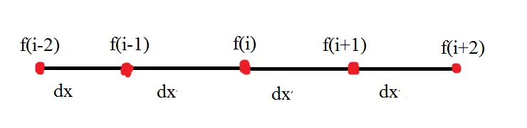
figure 1 : grid points of central difference scheme
`(triangle x^2. d^2f)/dx^2 = a. f(i-2)+b.f(i-1)+c.f(i)+d.f(i+1) + e.f(i+2)`........(3) ( Genral hypothesis equation for 4 th oder central difference scheme )
in oder to find out d^2(f)/dx^2 we have to find out the co-effecients a,b,c,d,e . This can be done using a taylors table , before that we have to find out the values for grid points f(i-2).
`f(i-1) = f(x) - f'(x).(triangle x)/(1!)+ f''(x).(triangle x^2)/(2!) - f'''(x).(triangle x^3)/(3!)......`.......(4) taylor's series expansion
as the same way in the eq (4) we have to find out the taylor's series expansion for all the other points in the Figure 1 . and substitute the co -effecients in the taylors table .
`triangle x =` The distance between the the grid point from f(i) , the distance is dx between two points .
|
stencil |
`f(i)` | `f'(i)triangle x` | `f''(i) triangle x^2` | `f'''(i) triangle x^3` | `f''''(i) triangle x^4` |
| f(x-2) | a | -2a | 2a | -4a/3 | 2a/3 |
| f(x-1) | b | -b | b/2 | -b/6 | b/24 |
| f(x) | c | 0 | 0 | 0 | 0 |
| f(x+1) | d | d | d/2 | d/6 | d/24 |
| f(x+2) | e | 2e | 2e | 4e/3 | 2e/3 |
| 0 | 0 | 1 | 0 | 0 |
Table 1 : Taylors table for 4th oder approximation of 2 nd oder derrivative in central difference scheme
since we have 5 points we need five stencils and the expansion of the stencil till `triangle x^4` and since we are finding out the 2 nd oder derrivative we are equation the other terms to 0 ( ie we are equating f ' , f ''' , f '''' to 0 ) and the f '' expansion terms to 1 . as shown in the table 1 . The equations for finding out the co-effecients are as follows :
`a+b+c+d+e = 0`.........(5)
`-2a-b+0+d+2e =0`.......(6)
`2a +b/2 + 0 +d/2 +2e = 1`....(7)
`-4a/3 -b/6 + 0 + d/6 + 4e/3 = 0`.....(8)
`2a/3 +b/24 +0 + d/24 + 2e/3 = 0`.....(9)
Now solving the four equations , we can find out the value of co-effecients of a, b,c , d and e . This can be done using a Matlab program for solving it with more ease figure 2 and 3 shows the program and value of co-effecients .
close all
clear all
clc
 a = [1 1 1 1 1; -2 -1 0 1 2 ; 2 0.5 0 0.5 2 ; -4/3 -1/6 0 1/6 4/3 ; 2/3 1/24 0 1/24 2/3 ]
 c = [ 0 ; 0 ; 1 ; 0 ; 0 ]
 b = inv(a)*c
Figure 2 : program to solve the central difference equation
a =

    1.0000    1.0000    1.0000    1.0000    1.0000
   -2.0000   -1.0000         0    1.0000    2.0000
    2.0000    0.5000         0    0.5000    2.0000
   -1.3333   -0.1667         0    0.1667    1.3333
    0.6667    0.0417         0    0.0417    0.6667


c =

     0
     0
     1
     0
     0


b =

   -0.0833
    1.3333
   -2.5000
    1.3333
   -0.0833

>>
Figure 3: solution for the co-effecients of the central difference scheme
a_1 = -1/12
b_1 = 4/3
c_1 = -5/2
d_1 = 4/3
e_1 = -1/12
`cds = (a*f(x-2dx)+ b*f(x-dx) + c*f(x) + d*f(x+dx) + e*f(x+2dx))/dx^2`...................(10)
substituting the function in eq 1 to eq 10 we get
`cds = ( a*(exp(x-2*dx)*cos(x- 2*dx)) + b*(exp(x-dx)*cos(x-dx)) + c*(exp(x)*cos(x)) + d*(exp(x+dx)*cos(x+dx)) + e*(exp(x+2*dx)*cos(x+2*dx)))/dx^2`......(11)
eq 11 is used in the program to evaluate the central difference sheme for a variable range of dx , the values of the co-effecients a,b,c,d&e is obtained from the figure 3 respectively .
Right hand skewed scheme or Forward difference scheme :
The objective of this part is to find out a 4 th oder forward difference scheme or Right handed skewed scheme for a 2 nd oder derrivative . In oder to find out the number of points or mesh elements in the equation we are using a formula
p+q = No of points for forward difference or right hand skewed scheme
p - oder of approximation
q - oder of derrivative
so for a 4 th oder approximation in a Right handed skewed scheme there are 6 points and the distance between each point is dx as shown in the figure 4.
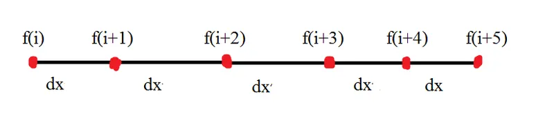
Figure 4 : Grid points for forward difference scheme
`triangle x^2.(d^2f)/dx^2 = a.f(i) + b.f(i+1) + c.f(i+2) + d.f(i +3) + e. f(i+4) + f. f(i+5)`................(8) ( Forward difference hypothesis equation )
in oder to find out d^2(f)/dx^2 we have to find out the co-effecients a,b,c,d,e . This can be done using a taylors table , before that we have to find out the values for other grid points:
`f(i+1) = f(x) + f'(x).(triangle x)/(1!)+ f''(x).(triangle x^2)/(2!) + f'''(x).(triangle x^3)/(3!)`.......so on .....(9) ( Taylors series expansion for f(i+1) )
as the same way in the eq (9) we have to find out the taylor's series expansion for all the other points in the Figure 4 . and substitute the co -effecients in the taylors table .
`triangle x =` The distance between the the grid point from f(i) , the distance is dx between two points .
|
stencil |
`f(i)` | `f'(i)triangle x` | `f''(i) triangle x^2` | `f'''(i) triangle x^3` | `f''''(i) triangle x^4` | `f'''''(i) trianglex^5` |
| f(x) | a | 0 | 0 | 0 | 0 | 0 |
| f(x+1) | b | b | b/2 | b/6 | b/24 | b/120 |
| f(x+2) | c | 2c | 2c | 4c/3 | 2c/3 | 4c/15 |
| f(x+3) | d | 3d | 9d/2 | 9d/2 | 27d/8 | 81d/40 |
| f(x+4) | e | 4e | 8e | 32e/3 | 32e/3 | 128e/15 |
| f(x+5) | f | 5f | 25f/2 | 125f/6 | 625f/24 | 625f/24 |
| 0 | 0 | 1 | 0 | 0 | 0 |
Table 2 : Taylors table for fourth oder approximation in Right handed skewed scheme
since we have 6 points we need five stencils and the expansion of the stencil till `triangle x^5` and since we are finding out the 2 nd oder derrivative we are equation the other terms to 0 ( ie we are equating f ' , f ''' , f '''' to 0 ) and the f '' expansion terms to 1 . as shown in the table 1 . The equations for finding out the co-effecients are as follows :
`a+b+c+d+e+f = 0`.......(12)
`0 + b+2c+3d+4e+5f = 0`.............(13)
`0 + b/2 + 2c + 9d/2 + 8e + 25 f/2 =1`..............(14)
`0 + b/6 + 4c/3 + 9d/2+32e/3 +125f/6 = 0`.........(15)
`0 + b/24 + 2c/3 + 27d/8 + 32 e/3 + 625f/24 = 0`....................(16)
`0 + b/120 + 4c/15 +81d/40 + 128 e/15 + 625 f/24 = 0`............(17)
eq 10 -15 can be solved by forming a matrix using MATLAB as shown in the figure 5 & 6 .
% forward differencing scheme matrix solving
close all
clear all
clc
a = [ 1 1 1 1 1 1 ; 0 1 2 3 4 5 ; 0 0.5 2 9/2 8 25/2 ; 0 1/6 4/3 9/2 32/3 125/6 ; 0 1/24 2/3 27/8 32/3 625/24 ; 0 1/120 4/15 81/40 128/15 625/24 ]
c = [ 0 ; 0 ; 1 ; 0 ; 0 ; 0 ]
b = inv(a)*c
Figure 5 : Program to solve the forward difference matrix
a =

    1.0000    1.0000    1.0000    1.0000    1.0000    1.0000
         0    1.0000    2.0000    3.0000    4.0000    5.0000
         0    0.5000    2.0000    4.5000    8.0000   12.5000
         0    0.1667    1.3333    4.5000   10.6667   20.8333
         0    0.0417    0.6667    3.3750   10.6667   26.0417
         0    0.0083    0.2667    2.0250    8.5333   26.0417


c =

     0
     0
     1
     0
     0
     0


b =

    3.7500
  -12.8333
   17.8333
  -13.0000
    5.0833
   -0.8333

>>
Figure 6 : Matrix and co -effecient values for forward difference scheme
so the co-effecient values are :
a_1 = 15/4
b_1 = -77/6
c_1 = 107/6
d_1 = -13
e_1 = 61/12
f_1 = -5/6
Note: we are taking the co-effecients in the form of fractions to reduce the round- off error
`fds = (a_1*f(x)+b_1*f(x+dx)+c_1*f(x+2dx)+d_1*f(x+3dx)+e_1*f(x+4dx)+f_1*f(x+5dx))/dx^2`...........(18)
substituting the function in eq 1 to eq 18 we get
`fds = (a_1*(exp(x)*cos(x)) + b_1*(exp(x+dx)*cos(x+dx)) + c_1*(exp(x+2*dx)*cos(x+2*dx)) + d_1*(exp(x+3*dx)*cos(x+3*dx)) + e_1*(exp(x+4*dx)*cos(x+4*dx))+ f_1*(exp(x+5*dx)*cos(x+5*dx)))/dx^2 ;`...(19)
eq 19 is used in the program to evaluate the fourth oder forward difference sheme for a variable range of dx , the values of the co-effecients a_1,b_1,c_1,d_1,e_1 & f_1 is obtained from the figure 6 respectively .
Left hand skewed scheme or Back ward difference scheme :
The objective of this part is to find out a 4 th oder Backward difference scheme or left handed skewed scheme for a 2 nd oder derrivative . In oder to find out the number of points or mesh elements in the equation we are using a formula
p+q = No of points for forward difference or right hand skewed scheme
p - oder of approximation
q - oder of derrivative
so for a 4 th oder approximation in a Left handed skewed scheme there are 6 points and the distance between each point is dx as shown in the figure 7.
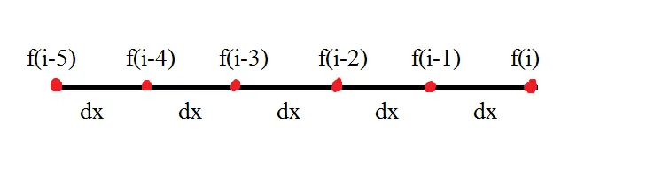
Figure 7 : Left handed skewed shceme grid points
`triangle x^2.(d^2f)/dx^2 = a.f(i) + b.f(i-1) + c.f(i-2) + d.f(i -3) + e. f(i-4) + f. f(i-5)`.........................(20) ( left handed skewed scheme hypothesis equation )
in oder to find out d^2(f)/dx^2 we have to find out the co-effecients a,b,c,d,e . This can be done using a taylors table , before that we have to find out the values for other grid points:
`f(i-1) = f(x) - f'(x).(triangle x)/(1!)+ f''(x).(triangle x^2)/(2!) - f'''(x).(triangle x^3)/(3!)`......... and so on .......(21) ( taylors series expansion)
as the same way in the eq (21) we have to find out the taylor's series expansion for all the other points in the Figure 4 . and substitute the co -effecients in the taylors table .
`triangle x =`The distance between the the grid point from f(i) , the distance is dx between two points .
|
stencil |
`f(i)` | `f'(i)triangle x` | `f''(i) triangle x^2` | `f'''(i) triangle x^3` | `f''''(i) triangle x^4` | `f'''''(i) trianglex^5` |
| f(x) | a | 0 | 0 | 0 | 0 | 0 |
| f(x-1) | b | -b | b/2 | -b/6 | b/24 | -b/120 |
| f(x-2) | c | -2c | 2c | -4c/3 | 2c/3 | -4c/15 |
| f(x-3) | d | -3d | 9d/2 | -9d/2 | 27d/8 | -81d/40 |
| f(x-4) | e | -4e | 8e | -32e/3 | 32e/3 | -128e/15 |
| f(x-5) | f | -5f | 25f/2 | -125f/6 | 625f/24 | -625f/24 |
| 0 | 0 | 1 | 0 | 0 | 0 |
Table 3 : Taylors table for left handed skewed scheme
from the figure 8 we can say that the right handed skewed and left handed skewed scheme is same for a second oder derrivative , this can be seen more clearly if we arrange the equations as shown eq (22-23)
`a+b+c+d+e+f = 0`.......(22)
`-(0 + b+2c+3d+4e+5f )= 0`.............(23)
`0 + b/2 + 2c + 9d/2 + 8e + 25 f/2 =1`..............(24)
`-(0 + b/6 + 4c/3 + 9d/2+32e/3 +125f/6) = 0`.........(25)
`0 + b/24 + 2c/3 + 27d/8 + 32 e/3 + 625f/24 = 0`....................(26)
`-(0 + b/120 + 4c/15 +81d/40 + 128 e/15 + 625 f/24 = 0)`............(27)
so the Matrix and the co -eefecient values are same as shown in figure 5 and 6
the co-effecient values are :
a_1 = 15/4
b_1 = -77/6
c_1 = 107/6
d_1 = -13
e_1 = 61/12
f_1 = -5/6
`bds = (a_1*f(x)+b_1*f(x-dx)+c_1*f(x-2dx)+d_1*f(x-3dx)+e_1*f(x-4dx)+f_1*f(x-5dx))/dx^2`...........(28)`
substituting the function in eq 1 to eq 28 we get the following expansion for the left handed skewed scheme , which is as follows :
`bds = (a_1*(exp(x)*cos(x)) + b_1*(exp(x-dx)*cos(x-dx)) + c_1*(exp(x-2*dx)*cos(x-2*dx)) + d_1*(exp(x-3*dx)*cos(x-3*dx)) + e_1*(exp(x-4*dx)*cos(x-4*dx))+
f_1*(exp(x-5*dx)*cos(x-5*dx)))/dx^2`........(29)
eq 29 is used in the program to evaluate the fourth oder left hand skewed sheme for a variable range of dx , the values of the co-effecients a_1,b_1,c_1,d_1,e_1 & f_1 is obtained from the figure 6 respectively .
MATLAB PROGRAM :
Proccedure :
1. create a separate function program to calculate the error due to central difference , right handed and left handed skewed 4 th oder schemes for a 2 nd oder derrivative.
2. calculate the analytical derrivative using the formula in eq 2 and give it as a input to the function program .
3. give the inputs of the co - effecients for the aproximation schemes as obtained from Figure 3 and 6
4. Now use the formulas obtained from eq (11) eq(19) and eq (29) to compute the central difference and skewed approximation schemes
5. Now compute for the output of the fuction program by coding for abs error = abs ( cds/fds/bds - Annalytical derrivative) respectively .
6. save thefunction program
7. In the Main program define the values of x and dx
8. Define the range of dx using the linspace command
9. now using the for loop compute the schemes and error for each values of dx , in simple words the output of the function program will change for the values of dx as dx will change from pi/4 to pi/400 with 100 intervals.
10 .example of the syntax for step 9 is as follows
for i = 1: length ( dx )
function_ output( i ) = taylors_table(x,dx(i))
11. now plot the out put errors of all the three schemes using a log log plot
12 . End the program
code :
% function program to calculate the errors using the 4th oder central difference ,forward difference and backward difference scheme for a second oder derrivative
% cds_error = central difference scheme error
% fds_error = forward difference scheme or right handed skewed scheme error
% bds_error = Backward difference scheme or left handed skewed scheme error
% given input
% fx) = exp(x)*cos(X)
function [ cds_error , fds_error , bds_error ] = taylor_table(x,dx)
Annalytical_derrivative = -2*sin(x)*exp(x);
% coeffecient values for central difference
a = -1/12;
b = 16/12;
c = -30/12;
d = 16/12;
e = -1/12;
% co-effecient values for Right handed and left handed skewed schemes
a_1 = 15/4;
b_1 = -77/6;
c_1 = 107/6;
d_1 = -13;
e_1 = 61/12;
f_1 = -5/6;
% central difference scheme
% cds = (a*f(x-2dx)+ b*f(x-dx) + c*f(x) + d*f(x+dx) + e*f(x+2dx))/dx^2
cds = (( a*(exp(x-(2*dx))*cos(x- (2*dx))) + b*(exp(x-dx)*cos(x-dx)) + c*(exp(x)*cos(x)) +  d*(exp(x+dx)*cos(x+dx)) + e*(exp(x+(2*dx))*cos(x+(2*dx))))/(dx^2)) ;
% Forward difference scheme
% fds = (a_1*f(x)+b_1*f(x+dx)+c_1*f(x+2dx)+d_1*f(x+3dx)+e_1*f(x+4dx)+f_1*f(x+5dx))/dx^2
fds = ((a_1*(exp(x)*cos(x)) +  b_1*(exp(x+dx)*cos(x+dx)) + c_1*(exp(x+2*dx)*cos(x+2*dx)) + d_1*(exp(x+3*dx)*cos(x+3*dx)) + e_1*(exp(x+4*dx)*cos(x+4*dx))+ f_1*(exp(x+5*dx)*cos(x+5*dx)))/(dx^2)) ;
% bds = (a_1*f(x)+b_1*f(x-dx)+c_1*f(x-2dx)+d_1*f(x-3dx)+e_1*f(x-4dx)+f_1*f(x-5dx))/dx^2
bds = ((a_1*(exp(x)*cos(x))+b_1*(exp(x-dx)*cos(x-dx))+ c_1*(exp(x-2*dx)*cos(x-2*dx))+ d_1*(exp(x-3*dx)*cos(x-3*dx))+ e_1*(exp(x-4*dx)*cos(x-4*dx))+ f_1*(exp(x-5*dx)*cos(x-5*dx))) /(dx^2)) ;
% error
cds_error = abs(cds - Annalytical_derrivative);
fds_error = abs(fds - Annalytical_derrivative);
bds_error = abs(bds - Annalytical_derrivative);
Figure 8 : Function program
close all
clear all
clc

x = pi/3 ;
dx = linspace(pi/4,pi/400,100);
for i = 1: length(dx)
    [cds_error(i),fds_error(i),bds_error(i)] = taylor_table(x,dx(i));
end
 loglog(dx,cds_error,'r')
 hold on
 loglog(dx,fds_error,'b')
 hold on
 loglog(dx,bds_error,'g')
 hold off
 hold off
 grid on
 legend('central difference scheme',' forward difference scheme ','Backward difference scheme')
 axis([10^-2 10^0 10^-10 10^3])
 xlabel('dx grid size')
 ylabel('error')
 title(' error vs dx for 4th oder aproximation of 2 nd oder derrivative for all the three schemes ')
Figure 9 : Main program
RESULTS AND CONCLUSION :
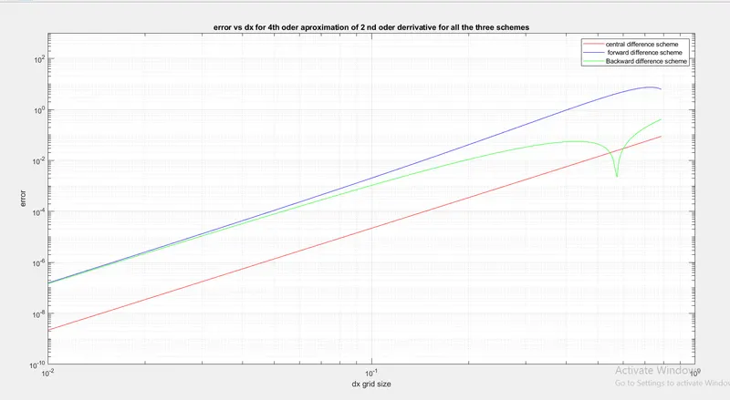
Figure 10 : error of 4 th oder schemes vs grid size
From the Figure 10 we can see that the error value of the 4 th oder central difference scheme is lesser then the errors due to the skewed scheme this is because the central difference scheme takes the input from the points on either side of the function f(i) where as the skewed scheme gets input from a single direction . The central difference scheme is more accurate but cant be used in all situations , for example we have to calculate the flow in a pipe , In this case , the flow is in a particular direction so we cant use the central difference scheme , only the skewed scheme can be used for approximations.
lets look at the conclusions more specificly :
1. The error due to central oder scheme is lower .
2. The rise in the error for the left handed and Right handed skewed scheme is linear and increases propotionally with the increase in the grid size .
3. The error in the left handed skewed scheme drops down suddenly at a higher grid size and again increases suddenly forming a inverse peak as shown in figure 10 due to Instability criterion.