Project 1 - Parsing NASA thermodynamic data
TITLE : FILE PARSING
AIM : To extract the 14 co -effecients from the NASA data file to find out the following :
1. To find out (i) Specific heat (ii) Enthalpy (iii) Entropy and plot the corresponding graphs with Temprature respectively
2. To find out the Molecular weight of all the 53 species and display it in the command window
3. Save all the three plots for the individual species respectively in each individual folders
INTRODUCTION :
Parsing in computer language means that a method which is used to collect and read a data from the given data file , this technique is used by the research scholars to get a particular set of data from a given data set . In this project we are going to look after the code that helps us to achieve the objective of the program . The formula used to calculate the Specific heat , Enthalpy and Entropy as shown in Figure 1.
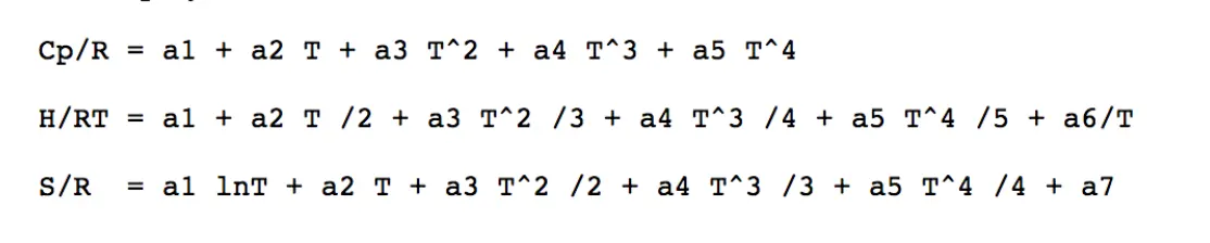
Figure 1 : The formulas used to compute the Specific heat , Enthalpy and Entropy
Matlab commands :
clc : Clears all the Input and Output from the command window
clear all : Removes the previously stored data from the code and work space
close all : Deletes the current figure and plots
strcat : for example t = strcat( s1, s2,s3) combines the corresponding row of characters
str2double : str2double converts the text in str to double precission , the syntax can be represented as X = str2double(str) if str is a character vector or string scalar then X is a numeric scalar
strcmp: The function " strcmp" is used when there is a need of comparission of two strings , The function takes the two input arguments (strings) and returns either true or false , same as the boolean operation
gcf : This command is used to get the frames
cd../ : This command changes the current folder into new folder
fopen : Opens the file name for read acess
fgetl : line = fgetl(file) , reads the first line of the data file
strfind : To find a specific string in a specifc line , for example " location_1 = strfind(line_7,'E'); " the location of the string " E " is assigned to the variable Location_1 .
strsplit : splits the variable or string with a delimiter such as ' ' .
mkdir : creates the file with the desired name in the current directory where the Matlab file exists , the syntax is as follows " mkdir(dir_name)" , dir_name is a variable in which the name of the file is stored
saveas : The command line is used to save the plots .
MATLAB PROGRAM :
Objective :
To extract the 14 co -effecients from the NASA data file to find out the following :
1. To find out (i) Specific heat (ii) Enthalpy (iii) Entropy and plot the corresponding graphs with Temprature respectively
2. To find out the Molecular weight of all the 53 species and display it in the command window
3. Save all the three plots for the individual species respectively in each individual folders
Steps :
In oder to achieve the objective of the program we have to follow the following outline
1. To develop a main code to read the data file and extract all the forteen co -effecients
2. Write a code for the function program to evaluate the Entropy
3. Write a code for the function program to evaluate the Enthalpy
4. Write a code for the function program to evaluate the specific heat
5. Write a code for the function program to evaluate the Molecular weight for each species and display it in the command window
6. Write a code for the function program to plot the graph for Enthalpy , Entropy and Specific heat vs Temperature respectively andf save the files in separate location
7. Calling all the five functions in the Main program
Main program code :
Proccedure :
1. Use the clear all , close all and clc command to clear the stored data from the workspace and command window .
2. open the file using the fopen command
3. Now we have to read the first five lines and skip them , this is done using the fgetl command and for loop
4. Now we have extract the data for the 53 species that is done by entering into the for loop .
5. The species name is collected using fgetl command and stored in a variable .
6. The temperature data from the line 6 is extracted using the strsplit, fgetl command , the value of temperature is evaluated by determining the position of the string , since the command line is in for loop the temperature data for all the 53 species is collected and stored in the respective variables.
7. The temperature data is divided using the linspace command
8. Now extracting the 14 co-effecients for each species from the data following the same proccedure as step 6.
9. calling the function programs for Enthalpy , Entropy and Molecular weight and Plots and saving the data .
10. Terminating the for loop using end command.
Code :
% PROJECT : FILE PARSING OF NASA THERMODYNAMIC DATA
% TO PLOT CP VS TEMPRATURE, ENTHALPY VS TEMPRATURE AND ENTROPY VS TEMPRATURE
% FINDING OUT THE MOLECULAR WEIGHT FOR ALL THE SPECIES
% SAIVING ALL THE PLOTS IN EACH INDIVIDUAL FOLDERS
% DONE BY G. SHIVA SAM KUMAR
close all
clear all
clc
% Universal gas constant ( unit R = J.mol^-1.k^-1)
R = 8.3145 ;
% First we have to read the data in the file and assign it to an variable
file_1 = fopen('NASA DATA.dat');
% Reading the First line of the file
fgetl(file_1);
% The first line of the file represents the global temperature
Global_temperature = fgetl(file_1);
temp = strsplit(Global_temperature,' ');
global_min_temp = str2double(temp{2});
global_mid_temp = str2double(temp{3});
global_max_temp = str2double(temp{4});
% Defining the temperature Range
temperature = linspace(global_min_temp,global_max_temp,300);
% Now entering the for loop
% using the for loop to skip the First three lines
 disp(' MOLECULAR WEIGHT OF ALL THE 53 SPECIES ')
for i = 1:3
   line1_5 = fgetl(file_1);
end
for j = 1: 53
   % Now to get the first line of the first species
   line_6 = fgetl(file_1);
   % separating the first line by the deleminator
   a = strsplit(line_6,' ');
   % getting the species name
   species_name = (a{1});
   z = length(a);
   % Now to determine the local temperatures
   local_low_temp = str2double(a{z-3});
   local_mid_temp = str2double(a{z-2});
   local_high_temp = str2double(a{z-1});

   % local temperature range of the species is defined using the linspace command
   local_temp_range = linspace(local_low_temp,local_high_temp,250);
   % Now extracting the forteen co-effecients of the thermodynamic data
   line_7 = fgetl(file_1);
   % Finding the location of the 'E' string
   location_1 = strfind(line_7,'E');
   % Finding all the co-effecients in the first line of the data
   c1 = str2double(line_7(1:location_1(1)+3));
   c2 = str2double(line_7(location_1(1)+4:location_1(2)+3));
   c3 = str2double(line_7(location_1(2)+4:location_1(3)+3));
   c4 = str2double(line_7(location_1(3)+4:location_1(4)+3));
   c5 = str2double(line_7(location_1(4)+4:location_1(5)+3));
   % Now the next set of co effecients
   line_8 = fgetl(file_1);
   location_2 = strfind(line_8,'E');
    c6 = str2double(line_8(1:location_2(1)+3));
    c7 = str2double(line_8(location_2(1)+4:location_2(2)+3));
    c8 = str2double(line_8(location_2(2)+4:location_2(3)+3));
    c9 = str2double(line_8(location_2(3)+4:location_2(4)+3));
    c10 = str2double(line_8(location_2(4)+4:location_2(5)+3));

    % Now to get the other set of co-effecients
    line_9 = fgetl(file_1);
    location_3 = strfind(line_9,'E');
    c11 = str2double(line_9(1:location_3(1)+3));
    c12 = str2double(line_9(location_3(1)+4:location_3(2)+3));
    c13 = str2double(line_9(location_3(2)+4:location_3(3)+3));
    c14 = str2double(line_9(location_3(3)+4:location_3(4)+3));

    % calling the specific heat function
    c_p = specific_heat( c1,c2,c3,c4,c5,c8,c9,c10,c11,c12,R,local_temp_range,global_mid_temp);
    % calling the enthalpy function
    H = enthalpy(c1,c2,c3,c4,c5,c6,c8,c9,c10,c11,c12,c13, R,local_temp_range,global_mid_temp);
    % calling the entropy function
    S = entropy(c1,c2,c3,c4,c5,c7,c8,c9,c10,c11,c12,c14,R,local_temp_range, global_mid_temp);
    % calling the molecular weight function
    mw(i) = molecular_weight(species_name);
    x = sprintf('%s_%d',species_name,mw(i));
    disp(x);
    % calling the plotting function
    plotting( c_p , H , S , local_temp_range , species_name);

end
fclose(file_1);
Figure 2 : Code for the Main program
Function program 1 : To find out the Specific heat of the species
The first seven co-effecients of the elements are used for the low temperature range and the next seven co-effecients are used for the high - temperature range , this is done using the if and else command the temperature value for each species is collected using the linspace command and stored in a variable " local_temp_range" , this variable is compared with the global mid temperature to find out the lower temperature range and higher temperature range . The formulas are used respectively to find out the specific - heat of the elements for higher and lower temperature range .
code :
% To create a function program for c_p (specific heat)
% For temperature greater then global mid temperature the first 7 coeffecients are used
% For temperature lower then global mid temperature the second 7 coeffecients are used
function [c_p] = specific_heat( c1,c2,c3,c4,c5,c8,c9,c10,c11,c12,R,local_temp_range,global_mid_temp)
if local_temp_range<=global_mid_temp
    c_p = R*(c1+c2.*local_temp_range + c3.*(local_temp_range.^2)+ c4.*(local_temp_range.^3) + c5.*(local_temp_range.^4));
else
    c_p = R*(c8+c9.*local_temp_range + c10.*(local_temp_range.^2)+ c11.*(local_temp_range.^3) + c12.*(local_temp_range.^4));
end
Figure 3 : Function program to compute the Specific - Heat of species
Function program 2 : To find out the Enthalpy of the species
The first seven co-effecients of the elements are used for the low temperature range and the next seven co-effecients are used for the high - temperature range , this is done using the if and else command the temperature value for each species is collected using the linspace command and stored in a variable " local_temp_range" , this variable is compared with the global mid temperature to find out the lower temperature range and higher temperature range . The formulas are used respectively to find out the Enthalpy of the elements for higher and lower temperature range .
Code :
% function program for evaluating the enthalpy from the NASA species data
function [H] = enthalpy(c1,c2,c3,c4,c5,c6,c8,c9,c10,c11,c12,c13, R,local_temp_range,global_mid_temp)
if local_temp_range<=global_mid_temp
    H = R.*local_temp_range.*( c1 + c2.*(local_temp_range./2)+ c3.*((local_temp_range.^2)./3) + c4.*((local_temp_range.^3)./4) + c5.*((local_temp_range.^4)./5) + c6./local_temp_range);
else
     H = R.*local_temp_range.*( c8 + c9.*(local_temp_range./2)+ c10.*((local_temp_range.^2)./3) + c11.*((local_temp_range.^3)./4) + c12.*((local_temp_range.^4)./5) + c13./local_temp_range);
end
Figure 4 : Function program to compute the Enthalpy of species or elements
Function program 3 : To find out the Entropy of the species
The first seven co-effecients of the elements are used for the low temperature range and the next seven co-effecients are used for the high - temperature range , this is done using the if and else command the temperature value for each species is collected using the linspace command and stored in a variable " local_temp_range" , this variable is compared with the global mid temperature to find out the lower temperature range and higher temperature range . The formulas are used respectively to find out the Entropy of the elements for higher and lower temperature range .
Code :
% To compute the Entropy of all the species or Elements

function [S] = entropy(c1,c2,c3,c4,c5,c7,c8,c9,c10,c11,c12,c14,R,local_temp_range, global_mid_temp)

if local_temp_range<=global_mid_temp

    S = R * (c1.*log(local_temp_range) + c2.*local_temp_range + c3.*(local_temp_range.^2)./2 + c4.*(local_temp_range.^3)./3 + c5.*(local_temp_range.^4)./4 + c7);
else
    S = R * (c8.*log(local_temp_range) + c9.*local_temp_range + c10.*(local_temp_range.^2)./2 + c11.*(local_temp_range.^3)./3 + c12.*(local_temp_range.^4)./4 + c14);

end
Figure 4 : Function program to compute the Entropy of the species or elements
Function program 4 : To compute the Molecular weight of all the 53 species individually
From the data we can see clearly that all the 53 elements contain atleast any of these elements " {'H' 'C' 'N' 'O' 'AR'}" . The logic is very simple we have to use the atomic weight of these 5 elements to calculate the molecular weight of the the 53 species . This is dome using the for loop , strcmp, if and else command , lets put more light on the concept the value of i varies from 1: length of the species name and value of j varies from 1: length of atomic weights . The strcmp command line is used to compute the molecular weight .
Code :
% Function to compute and display Molecular weight of each elemts for all the 53 elements

function [weight] = molecular_weight(species_name)
   s = {'H' 'C' 'N' 'O' 'AR'};
   % Atomic weight of each elements
  atomic_weight = [ 1 12 14 16 40 ];
  weight = 0 ;
  for i = 1:length(species_name)
      for j = 1:length(s)
          if strcmp(species_name(i),s(j))
              weight = weight + atomic_weight(j);
              pos = j ;
          end
      end
      n = str2double(species_name(i));
      if n>1
          weight = weight + atomic_weight(pos)*(n-1);
      end
  end

end
Figure 5 : Function program to compute the Molecular weight of all the 53 species individually
Function program 5 : To compute a code to plot the variation of Specific heat , Enthalpy and Entropy with respect to Temperature and save the files in a seprate directories
The mkdir and cd../ command is used to save the files in respective directory and return back to the main default directory each time till the loop runs respectively. The plots are saved separately each time using the getframe command line and save as command line .
Code :
% FUNCTION PROGRAM TO PLOT THE GRAPHS AND SAVE THE FILE
function plotting ( c_p , H , S , local_temp_range , species_name)
dir_name = species_name ;
mkdir(dir_name) ;
cd(dir_name);
% plotting temperature vs specific heat
figure(1)
plot (local_temp_range, c_p, 'linewidth',3,'color','r');
title(sprintf(' Specific heat vs Temperature for %s:',species_name));
xlabel('temperature');
ylabel('specific heat');
saveas(gcf,'t_vs_cp.jpg')
% plotting temperature vs specific heat
figure(2)
plot (local_temp_range, H , 'linewidth',3,'color','b');
title(sprintf(' Enthalpy vs Temperature for %s:',species_name));
xlabel('temperature');
ylabel('Enthalpy');
saveas(gcf,'t_vs_enthalpy.jpg')
% plotting temperature vs specific heat
figure(3)
plot (local_temp_range,S, 'linewidth',3,'color','g');
title(sprintf(' Entropy vs Temperature for %s:',species_name));
xlabel('temperature');
ylabel('Entropy');
saveas(gcf,'t_vs_entropy.jpg')
% changing the folder to the previous folder
 cd ../ ;

end
Figure 6 : Function program to compute a code to plot the variation of Specific heat , Enthalpy and Entropy with respect to Temperature and save the files in a seprate directories
RESULTS :
The molecular weight of all the 53 elements are displayed in the command window as shown in Figure 7.
MOLECULAR WEIGHT OF ALL THE 53 SPECIES
O_16
O2_32
H_1
H2_2
OH_17
H2O_18
HO2_33
H2O2_34
C_12
CH_13
CH2_14
CH2(S)_14
CH3_15
CH4_16
CO_28
CO2_44
HCO_29
CH2O_30
CH2OH_31
CH3O_31
CH3OH_32
C2H_25
C2H2_26
C2H3_27
C2H4_28
C2H5_29
C2H6_30
CH2CO_42
HCCO_41
HCCOH_42
H2CN_28
HCN_27
HNO_31
N_14
NNH_29
N2O_44
NH_15
NH2_16
NH3_17
NO_30
NO2_46
HCNO_43
HOCN_43
HNCO_43
NCO_42
CN_26
HCNN_41
N2_28
AR_0
C3H8_44
C3H7_43
CH3CHO_44
CH2CHO_43
>>
Figure 7 : Molecular weight of all the 53 elements
The plots of Specific heat , Enthalpy and Entropy vs temprature for AR, C , H and CO2 respectively are shown from Figure 8 - 19 .
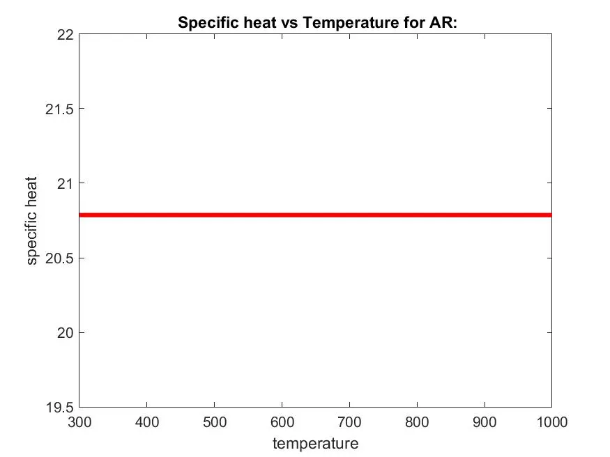
Figure 8 : cp vs t
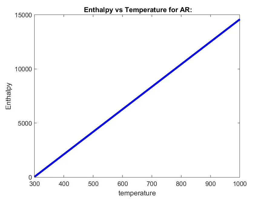
Figure 9 : H vs t
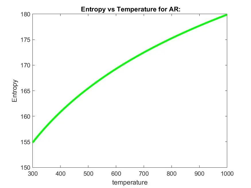
Figure 10 : S vs t
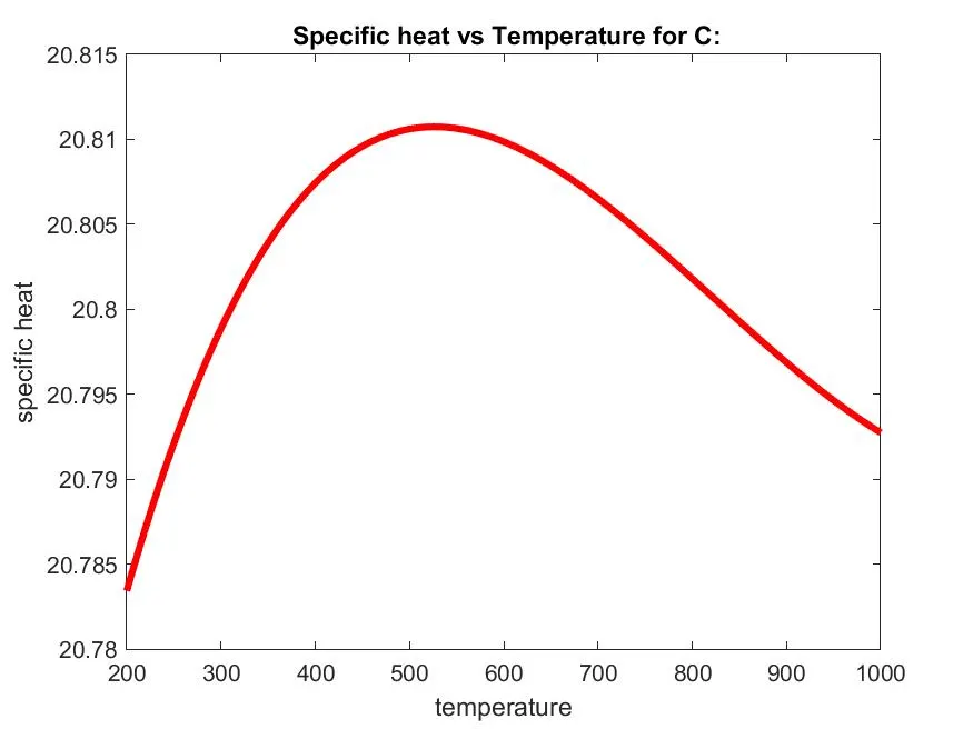
Figure 11 : cp vs t
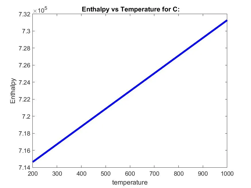
Figure 12 : H vs t
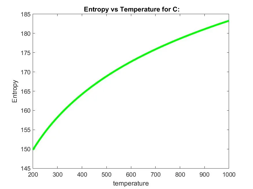
Figure 13 : S vs t
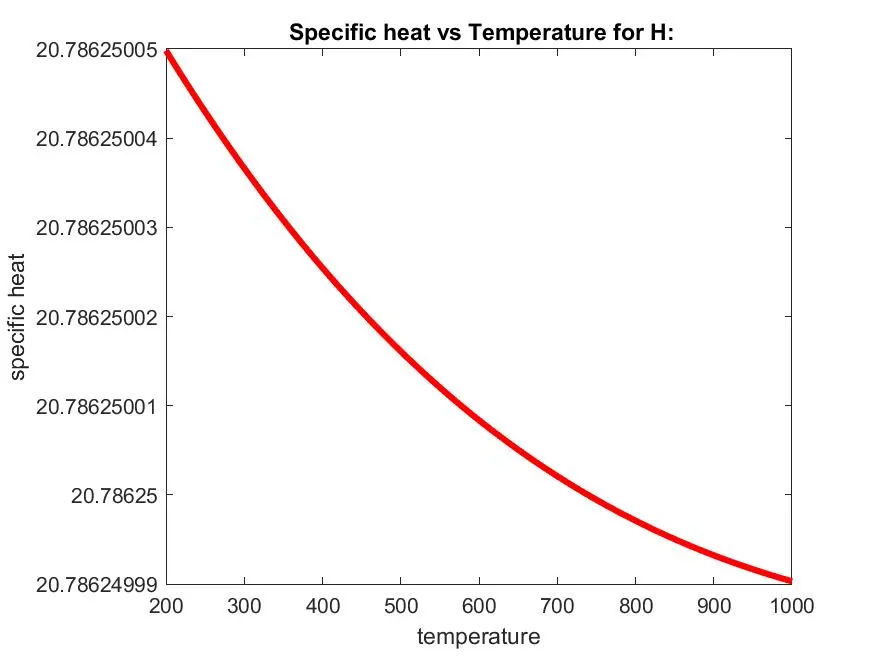
Figure 14 : cp vs t
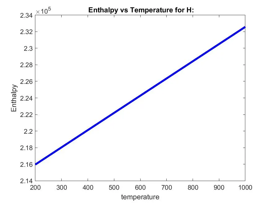
Figure 15 : H vs t
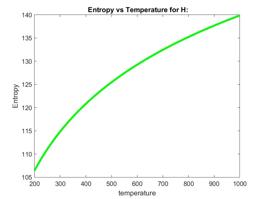
Figure 16 : S vs t
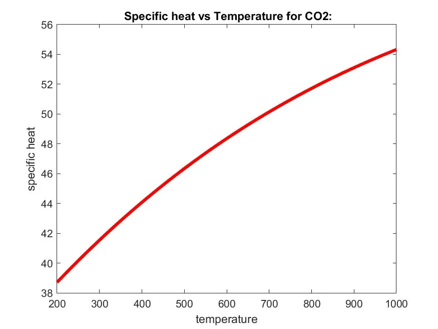
Figure 17 : cp vs t
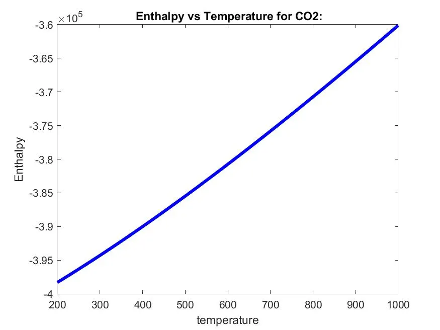
Figure 18 : H vs t
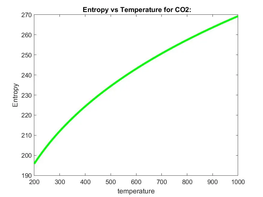
Figure 19 : S vs t
The files containing the plots respectively are stored sperately in diffrent directories as shown in Figure 20. There are total 53 folders and 159 files as shown in Figure 21.
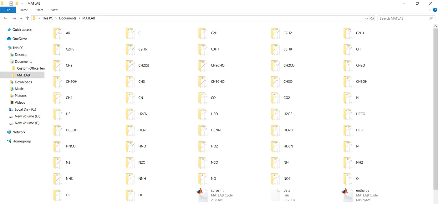
Figure 20 : Location containing the files for the respective plots of Specific heat , Enthalpy and Entropy of all the 53 elements
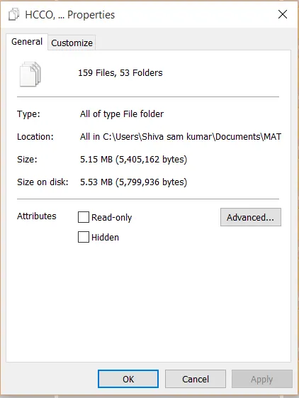
Figure 21 : Properties of the saved folders and files
-------------------------------------------------- END-------------------------------------------------------