Week 4 - Genetic Algorithm
AIM :
To write a code in MATLAB to optimise a stalgamite function and find out the global maxima
INTRODUCTION :
The main objective of this program is to understand the concept of optimisation and use it MATLAB to optimise a stalgamite function to find out the global maxima and global minima using genetic algorithm command in MATLAB . Stalgamite function model is just a model having a number of hills in it which makes it to look like stalgamite , here we are finding out the co- ordinates of the hill top in mathematical words can be said as maxima. In oder to achieve the objective we have to understand some basic concepts lerts have a look on them .
Optimisation :
In simple words optimisation can be explained as using the best or most effective use of situation or the resource , Lets understand this concept in mechanics in a better way for example we have a bracket and the problem is the max - von -misses stress is acting in the fillet region of the bracket this leads to the failure of the bracket over a shorter period of time for this optimisation method in finite element analysis is used , which basically finds out the best orientation of the fillet co-ordinates by performing a number of iterations by6 having a specifiv bounds or constraints , figure 1 shows an optimisation problem of a lug bracket with the constaraints and the objective.
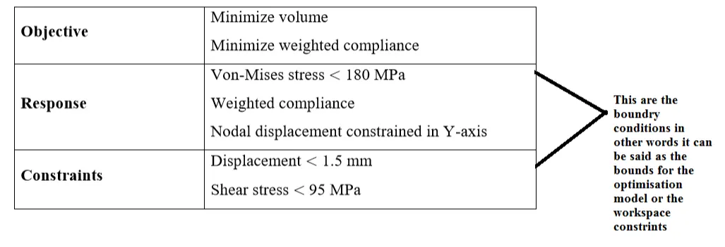
Figure 1 : example of an optimisation problem
Genetic Algorithm :
Genetic algorithm (ga) is a command used in MATLAB to perform the process of optimisation , this command basically performs a number of iterations validating the function and evaluating it and last gives the best and appropriation function based on the constraints . To understand the command lets put more light on the concep " genetic algorithm " . A genetic algorithm is a search that is inspired by charles darwins theory of Natural evolution . This algorithm reflects the process of natural selection where the fittest individuals are selected for reproduction ( ie second iteration) in oder to produce offspring of the neutral generation as shown in figure 2 .
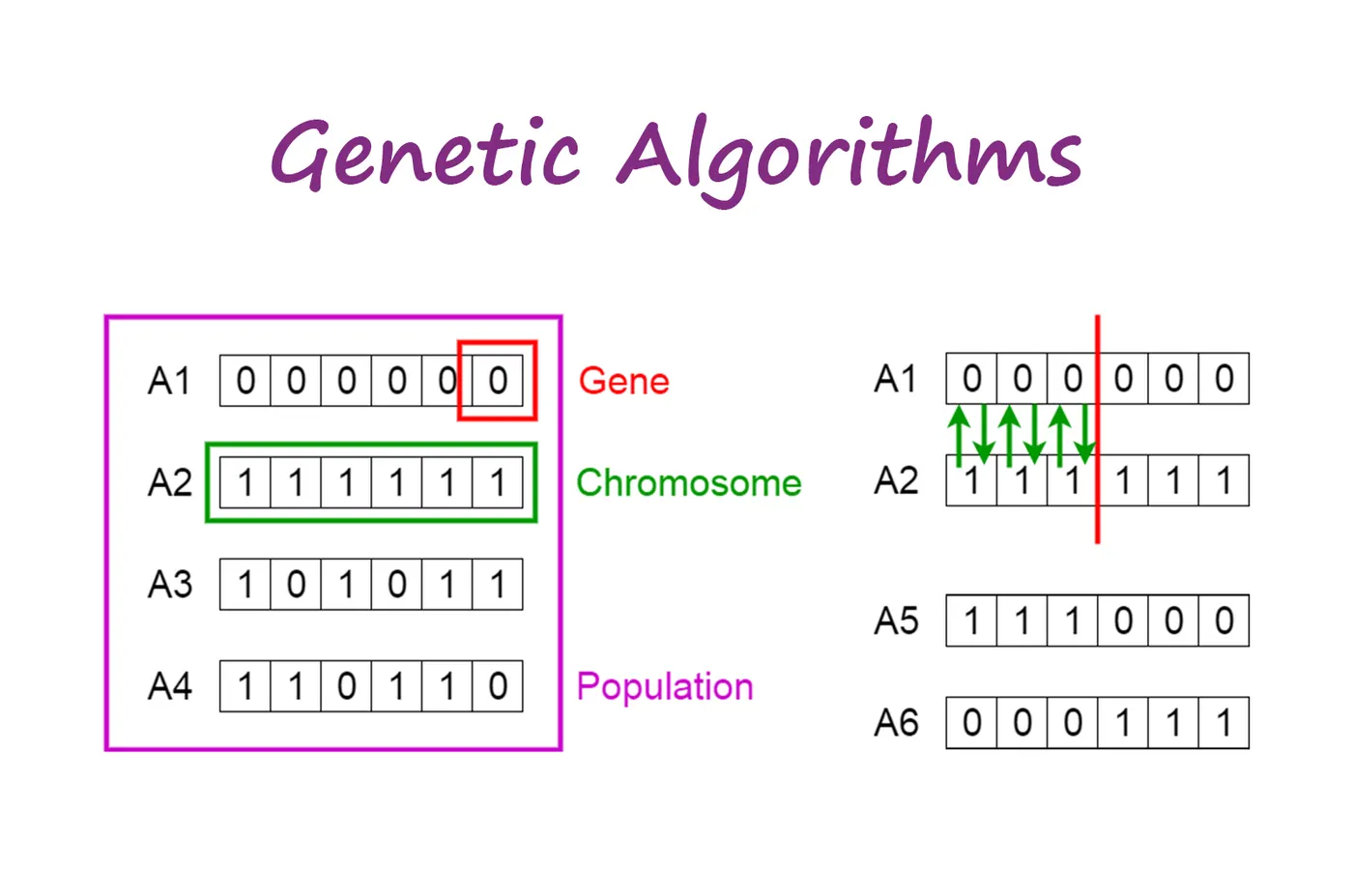
Figure 2 : genetic algorithm behaviour
The working structure of the ga command has been explained as follows :
1. The algorithm begins by creating a random initial population.
2. The algorithm then creates a sequence of new population . At each step , the algorithm uses the individuals in the current generation to create the next population . To create a new population the algorithm follows certain steps :
a). Scores each member of the current population by computing its fitness value , This values are called the raw fitness scores .
b). Scale the raw fitness scores to convert them into a more usable range of values , these values are known as expectation scaled values .
c). Selects members called parents based on the expected values
d). Some of the individuals in the current population that have a lower fitness value are chosen as elite individus , these elite individuals are passed on to the next population for valuation
e). Now childrens are produced from the parents . Childrens are produced either by the random changes of a single parent m,utation or by combining the vector entries of a pair of parents also known as cross over.
f). Replaces the current population with the children to form the next generation .
g). The algorithm stops when one of the stopping criteria is met
Five phases are considered in a genetic algorithm they are as follows :
1. Initial population
2. Fitness function
3. Selection
4. Cross over
5. Mutation
Initial population :
The process begins with a set of individuals which is also known as population , we get a n number of individuals and each individuals are the solution of the problem we want to solve . An individual is characterized by a set of parameters(variables) known as genes. Genes are joined into a string to form a chromosome ( ie solution).
In ga the set of genes of of an individual is represented using a string , in terms of an alphabet. Usually binary values are used . We say that we encode the genes in a chromosome.
Fitness function :
The fitness function determines how to fit an indidual( in simple words can be said as the ability of the individual to compete with the other individuals ) . It gives a fitness score to each individual. The probability that an individual will be selected for reproduction is based on the individuals fitness score.
Selection :
The idea of the selection phase is to select an fittest individual and let them pass their genes to the next genration
Cross- over :
Is the most significant phase in a genetic algorithm . Foe each pair of parents to be mated , a cross over poiny is chosen at a random process within the genes . Offsprings are created by exchanging the genes of parents among theem selves until the cross over point is reached . The new off springs are added to the population.
Mutation :
Mutuation occurs to maintain diversity and prevent premature convergence within a population
Termination :
The algorithm terminates if the population has converged ( does not produce off spring which are significantly different fromn the previous generation). Then it is said that the ga has provided a set of solutions to our problem.
Syntax :
In this project we are using the ga command line to optimise the stalagmite function lets look at the syntax :
[x fval] = ga(@fitnessfun,nvars,options ) where :
@fitnessfun = function handle ( here the stalagmite function )
nvars = is the number of independent variables for the fitness function
The results are given by
fval - Final value of the fitness function
x - point at which the value is attained
the function ga is used when you want the results to directly return to the workspace in the MATLAB
x = ga(fun, nvars,a,b,aeq,beq,lb,up,noncolon,intcount, options)
if no value exists the [] is used ; in this a,b,aeq,beq, noncolon and intcount values are not given so [] is used in the program
Global Maxima :
Global maxima also known as absolute maxima is the largest overall value of the se or function over the entire range . genetic algorithm (ga) in MATLAB is used for optimisation but it finds only the minima but the objective of thye program is to find out the maxima of the stalagmite function. we know that the global minima is equal to the -(global maxima ) so we can say that the global maxima = -(global minima ) . so in oder to the plot the maxima of the stalagmite function we are plotting the - ( optimized function result) .
PROGRAM :
Objective : To optimise the stalagmite model inoder to find out the global maxima of the function
Proccedure :
In oder to understand the concept of optimization and how to program it in MATLAB we have to go through three basic studies which clearly explains the proccedure to optimise the stalagmite function in a appropriate way to get a proper value for global maxima of the stalagmite function. The need for this study is because if we follow the genral proccedure without giving the bounded constraints we will get different results each time we run the program .
Function program :
In this matlab program we are using two sub programs (ie function programs) lets have a look at both of those programs :
Function program 1 : stalagmite
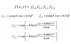
Figure 3: Is the stalagmite function
As shown in the Figure 3 we can see that the stalagmite function is varies as the function of two variables x&y , which is given as an input to the ga commandline used in MATLAB. All the variables f1_x,f2_x,f1_y & f2_y are computed together to derive the stalagmite function with respect to x & y as shown in the figure 3 .
Concept behind the code :
we are creating the function program so that we can call it in the main program , this program is created to define the stalagmite funcion f(x,y) . The idealogy behind the program is very simple as given in figure 3. We are assigning the values of f1_x ,f1_y,f2_x and f2_y to the variables f1_x,f1_y,f2_x and f2_y respectively and define the stalagmite function f (x,y) = f1_x*f1_y*f2_x*f2_y .
code :
function [F] = stalagmite(input_vector)
 x = input_vector(1)
 y = input_vector(2)

 f_1_x = (sin((5.1*pi*x)+0.5)).^6 ;
 f_1_y = (sin((5.1*pi*y)+0.5)).^6 ;
 f_2_x = exp((-4*log(2))*(x-0.00667).^2/0.64);
 f_2_y = exp((-4*log(2))*(y-0.00667).^2/0.64);

 F = -( f_1_x*f_1_y*f_2_x*f_2_y );

end
Figure 4 : Stalagmite function program code
Function program 2 : get_stalagmite
From figure 2 we can see clearly that for the stalagmite function we need two inputs in this function program we are going to define the two inputs as input(1) and input(2) , the obhective of this project is to plot the stalagmite function as a 3 -d plot to obtain the coordinates we are creating a matrix for x & y using the meshgrid command as shown in the figure 5 . this program is saved as " get_stalagmite " and is called when we call the stalagmite function , the inputs are assigned to f(i,j) the values of xx and yy are assigned to i and j respectively using the for loop and are called using the variable "f" ( ie remeber carefully it is small f and the stalagmite function is assigned to " F" capital f ) .
% to creat a function program for calling the stalagmite fuction in the main program
% create a mesh grid and assign it to the primary function using for loop
function [f] = get_stalagmite(x,y)
[xx,yy]= meshgrid(x,y);
 % creating the for loop

 for i = 1:length(xx)
 for j = 1:length(yy)
     input(1)=xx(i,j);
     input(2)=yy(i,j);
     f(i,j) = stalagmite(input);
 end
 end
end
Figure 5 : get_stalagmite function code
case 1:
After coding up the function program now we have to code the main program , In this project we are going to look on the three cases . Lets understand the main program code step by step
1. First use the close all , clear all and clc command to clear the work space and command window.
2. Define the variable x & y using the linspace command (ie , we are creating an array for x and y each having 200 equally space values from 0 to 0.6 )
3. Now defining the number of cases or in other words we are defining the number of iterations for the program to run (ie how many times the program need to run before computing the results .
4. Now assigning the get_stalagmite function to the variable " f" .
5. Now assigning the " f " ( small f ) to the the variable " F" ( capital f) and calling the function ( ie stalagmite function) , and assigning F= - f ( cause thje objective of the program is to find the global maxima and ga command line only finds out minima and we know that the negative of minima is the global maxima of the function or model ) .
6. Now using the for loop and ga command line we are assigning for cases 1to 150 to the variable "i" the i value changes respectively.
7. as explained in the syntax for the ga command lihne we are giving the stalagmite function handle and no of variables as the input for the command line and the out put of the command line is inputs and f val ( here the optimised results are assigned to the variable "fopt" ) , the command line is as follows " [inputs,fopt(i)] = ga(@stalagmite,2) " .
8. The fopt value changes with the variable i as for i = 1 to length(cases).
9. since we are finding out the maxima value we are plotting " - fopt " . using the plot command , shading interp command is used to smoothen the stalagmite plot. we are using the plot3 command to plot for xopt, yopt and fopt to plot the 3 plot .
10. For plotting all the variables we are using the hold on command . we are using the subplot command to plot the variance and optimisation clearly as shown in the outputs.
11. tic and toc commands are used to compute the working time of the program.
case 2 :
In case 2 we are assigning the workspace for the optimisation function . In this case we are applying the bounds for the maxima ie we are saying the program to compute the maxima within the bounds given as input . The proccedure for case 2 is same follow all the steps till step 6 , only the ga command line is moddified as follows " [inputs,fopt(i)]= ga(@stalagmite,2,[],[],[],[],[0;0],[0.6;0.6]) " . Here [0;0] & [0.6;0.6] are given as upper and lower bounds respectively. Rest all other steps are same for the study of statistical behiviour of the stalagmite function.
case 3 :
In case 3 we are assigning the population size to the genetic algorithm command line , the syntax for it is as follows :
1. " options = optimoptions('ga','populationsize',250) " .
2. Now assingn this options to the ga command line as shown " [inputs,fopt(i)]= ga(@stalagmite,2,[],[],[],[],[0;0],[0.6;0.6],[],[],options) " .
by doing this we can compute and plot the exact maxima of the stalagmite function .
The complete code for optimising the stalagmite function with the three case study are scripted as shown in Figure 6 .
close all
clear all
clc
% defining our search space using the linspace command
x = linspace(0,0.6,200);
y = linspace(0,0.6,200);
cases = 150;
% study 1 - statistical behaviour
f = get_stalagmite(x,y);
F = -f % to get the maxima value
tic
for i = 1:cases
    [inputs,fopt(i)] = ga(@stalagmite,2);
    xopt(i) = inputs(1);
    yopt(i) = inputs(2);
end
study_1_time = toc % used to find the run time
fopt = -fopt;
figure (1)
subplot(2,1,1)
hold on
surfc(x,y,F)
shading interp
plot3(xopt,yopt,fopt,'marker','O','markersize',5,'markerfacecolor','r')
title(' UNBOUNDED INPUTS ')
subplot(2,1,2)
plot(fopt)
xlabel(' ITERATIONS ')
ylabel(' FUNCTION MAXIMUM ')

% study 2 statistical behaviour with the upper and lower bounds
tic
for i = 1:cases
    [inputs,fopt(i)]= ga(@stalagmite,2,[],[],[],[],[0;0],[0.6;0.6]);
    xopt(i) = inputs(1);
    yopt(i) = inputs(2);
end
f= get_stalagmite(x,y)
F= -f
study_2_time = toc
fopt = -fopt;
figure(2)
subplot(2,1,1)
hold on
surfc(x,y,F)
shading interp
plot3( xopt,yopt,fopt,'marker','O','markersize',5,'markerfacecolor','r')
title(' BOUNDED INPUTS ' )
subplot(2,1,2)
plot(fopt)
xlabel('ITERATIONS')
ylabel(' FUNCTION MAXIMUM ')

% study 3 - Increasing the population size and iteration
options = optimoptions('ga','populationsize',250);
f = get_stalagmite(x,y);
F = -f
tic
for i = 1: cases
    [inputs,fopt(i)]= ga(@stalagmite,2,[],[],[],[],[0;0],[0.6;0.6],[],[],options);
    xopt(i) = inputs(1);
    yopt(i) = inputs(2);
end
fopt = -fopt ;
study_3_time = toc
figure(3)
subplot(2,1,1)
hold on
surfc(x,y,F)
shading interp
plot3(xopt,yopt,fopt,'marker','O','markersize',5,'markerfacecolor','r')
title(' BOUNDED INPUTS WITH INCREASED POPULATION SIZE ')
subplot(2,1,2)
plot(fopt)
xlabel('ITERATIONS')
ylabel(' FUNCTION MAXIMUM ')
Figure 6 : Full code of final program to optimise the stalagmite function
RESULTS AND DISCUSSIONS :
case 1 :
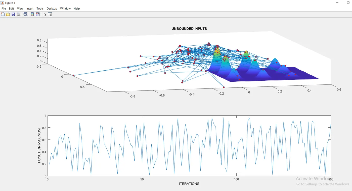
Figure 7 : Output for case 1 (unbounded inputs )
From figure 1 we can see that the ga command line plots the maxima or (fopt) all over the work space , the ga comand line computes the maxima but it has no bounds so the plot looks ugly for this we do the second statistical study or study 2 .
case 2 :
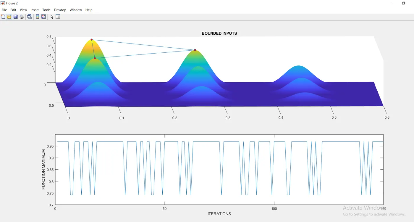
Figure 8 : Output plot for case 2
In case 2 we are specifiying the bounds ie upper and lower bound in simple words we can say the we are specifying a workspace for the program to compute the output as result we can see that in figure 8 we get a cleaner plot showing the Maxima of the stalagmite function.
Case 3 :
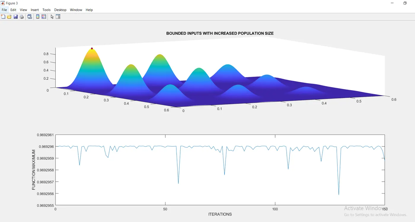
Figure 9 : Output plot for the case 3 with increase population size ( final result plotted down )
In oder to get a exact plot for the global maxima we can increase the population size with the bounded constraints. The exact point of Maxima is computed as shown in Figure 9 .
From all the three case studys we can conclude that for achieving a cleaner and exact result in an optimisation problem we have to follow these three steps :
1. Increase the iteration
2. Specify the Bounds lower and upper bounds
3. Increase the population size