Week 3 - Solving second order ODEs

AIM : To solve the ordinary differential equation (ODE) of an simple pendulum with damping and animating the pendulum .

INTRODUCTION :

Pendulum is a device which has been in existence from the ancient period and has been a base for solving a n- number of problems in engnieering . A pendulum is simply an string attached to a celieng with wight at its other end which works under the concept of newtons second law and the tangential force of the gravity. In oder to solve the ODE equation for pendulum we have to obtain an equation to solve the motion of the pendulum in oder to understand the motion of pendulum and the concept damping we have know about some basic terms which are :

1. Frequency : frequency of the pendulum can be defined as the number of times the pendulum moves forward and backwards

2. Amplitude : Amplitude of the pendulum can be defined as the horizental distance of the bob of the pendulum from the highest point to the line of equilibirium .

3. Time period : The time required by the pendulum to complete one complete swing is known as the time period.

Now lets solve the simple equation for the motion of the pendulum. The free body diagram of the pendulum swinging with a bob of mass m is as shown in figure 1.

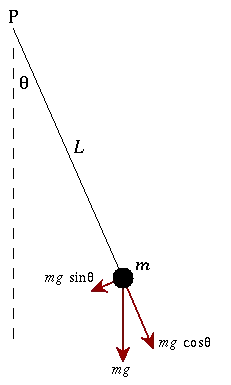
Figure 1 : The free body diagram of the pendulum

As we can see that the the tangential component of the the force due to gravity (mg) decides the displacement of the pendulum that is `mg sin(theta)`. The theta decides the displacement of the pendulum bob , the equation of motion for the pendulum can be expressed as shown :

`(d^2theta) /(dt)^2 + b/m*(d theta)/dt+ g/l*sin theta = 0` (1)

b = damping co-efficient or damping factor

m = mass of the bob

g = acceleration due to gravity

l = Length of the string connected to the pendulum

`theta =` The angle between the equlibirium line to the line of action of the string

In oder to stimulate the pendulum we have to determine the different position of the bob of the pendulum with respect to the time period, for that we have to solve the second oder equation , inoder to solve the second oder equation we have to simplify the second oder equation into into first oder equation as follows :

we know that the differential of the angular displacement is equal to the angular velocity, in oder to convert the second oder equation into first oder equation we have to do some assumptions such as :

`theta = theta_1` (2)

`(d theta_1)/dt = theta_2` (3)

`(d theta )/dt = ( d theta_1)/ dt = theta_2` ( which has been asumed as the angular velocity ) (4)

`(d^2 theta)/dt^2 = ( d^2 theta_1)/dt^2= (d theta_2)/dt` (5)

when we substitute the equation (2),(3),(4),(5) into equation we get

`(d theta_2)/dt = -b/m .theta_2 - g/l*sin theta_1` (6)

now theta value of `theta_1 ,theta_2` can be clubbed into a matrix `theta`

there fore [`theta`] = [ `theta_1 , theta_2`]

so , `d/dt [ theta_1 ;theta_2] = [ theta_2 ; -b/m*theta_2-g/l*sintheta_1]` (7)

and `theta_1 =` Agular displacement

`theta_2 =` Angular velocity

The change in `theta_1 & theta_2` with respect to change in time is has been obtained as the result which *kis in the form of 1*2 matrix which is one row and two column , the first column is the change in agular displacement with respect to time the second column is the change in the angular velocity with the time , the values obtaiined in the first column ie the change in displacement with respect to time is used to plot the position of the bob for the stimulation of the pendulum . The obtained results are plotted down to see the variation of the angular displacement5 and angular velocity.

MATLAB PROGRAM :

Objective : To plot the change in angular displacement and angular velocity with respect to time

Inputs :

damping factor (b) = 0.05

g = 9.81 m/s

length of the pendulum (l) = 1

m= 1 kg

Angular displacement and angular velocity when t= 0 is 0 and 3 rad/sec respectively.

The time period in this program is taken as 0- 20 sec

for our convinience in this program we are taking about 400 time intervals in between the time period of 0-20 sec ,which means we wil get our result output as a 400*2 matrix ie 400 rows and 2 columns .

Commands :

clear all : Removes all the data stored in the workspace and clears it

close all : Deletes all the current figure

clc : clears all the data stored in the command window

linspace(x,y,z) : creates an array of 1 row and z columns starting from x to y with equal intervals

function (x) = call_of_fuction( inputs of function, geometric inputs) : this command is basically used to call an function saved in a different program to other program for simplicity

hold on : When we are plotting the variance of two or more different factor in respect to single condition we need hold on command to differenciate .

pause( 0.03) :pause(0.3) = pauses the video for 0.03 seconds

m(ct)=getframe(ct)= stiches all the figure into a single variable(figure)=m , for animation

for loop = for loop command is basically used to repeat the same function to n number of variables

ct = plots are divided into different figures

ode45 = This command is used to solve an odinary differential equation. The syntax of the ode45 can be explained as below :

[ t, results] = ode45(@(t,theta) ode_func ( t, theta ,b , g , l, m ) , t_span, theta _0 )

ode_func ( t, theta ,b , g , l, m ) = The function which needs to be integrated (ie : in this program the function ode_func is an function of theta, l, m, b, g )

t_span = Time span for the ode function , In this program we have a time span from 0 to 20 sec .

theta( theta_0) = Is the intial condition

M(ct) = getframe(gcf) = This command is used to combine the different plots or frames into a single frame or movie (M).

VideoWriter = This command is used to save the video

writeVideo = This command is used to write the videofile in the video

end = This command is used to terminate the program

Proccedure :

In this program we have to code a plot to show the variance of angular displacement and angular velocity with respect to time and stimulate a pendulum for achieveing this objective we have to follow some steps which are as follows :

1.First use the clear all ,close all and clc command to clear the workspace and the command video.

2. Now we give the inputs to the program such as ( b, g, l , m and theta_0 ) , theta_0 is the input matrix which has the angular displacement and angular velocity

3. Now we are specifing the time interval using the linspace command by dividing the time period in to n number of equal intervals.

4. Now we are using the ode45 solver to solve the ordinary differential equation.

5. For solving the ode using ode45 solver we have to create a separate function which varies with the timeperiod .

6. In this function we are giving the ode as the input.

7. we are specifing the equations for `(d[ theta_1 and theta_2 ] )/ dt` and for theta1 and theta2

8. Now basically we call this function using the ode solver in the main program .

9. By using the ode solver we get an output of a matrix with [ time_ span, results ] , which means how the Angular displacement and Angular velocity varies with the variying time.

10. Now we are ploting this out put using the plot command and the first output of our program is achieved.

11. Now in oder to stimulate program we have to animate using the plot command by plotting the variance of the displacement with respect to time .

12. The end point of the string is attached with a bob the bob is created using the " marker " command and given a face width and face coloux .

13 . The string is defined with the co-ordinates [ x_start , y_start ] & [ x_end , y_end ] ; the x-end , y_end are the tangential component defined with theta , here theta is the solution array

for example : x_start = 0

y_start = 0

x_end = 1* sin (theta)

y_end = -1*cos(theta)

we know that our theta is a solution array of angular displacement and angular velocity to stimulate the pendulum we have to plot the different values of angular displacement with respect to time for the co-ordinates x_end and y_end . For this we are using the " for loop " .

14 . For each value of i the values of displacement (ie the first column of the result matrix ) varies from 1 . This values of i varies for different values of x_end and y_end this data is given as the feed to the for loop .

15. Now a counter is defined to generate various plots .

16. Now using the plot command we are plotting ( x_start ,y_start ) and (x_end, y_end ) , the later co-ordinate is assumed as the bob which is marked using an marker.

17. Now after plotting the co-ordinates we are using the " M(ct) = getframe(gcf) " to combine different frames into single frame to plot the stimulation video , the animateed video is stored to the system directory using the command " VideoWriter " , " videofile " and " writeVideo" command .

18 . Now the for loop is terminated using the end command and the program is saved and then "f5" key is pressed to run the program .

Code :

% To plot the change in displacement and tvelocity with respect to time 
% to stimulate a simple pendulum 
clear all
close all 
clc 

% inputs 
b = 0.05; 
l = 1;
g = 9.81;
m = 1 ;
 % initial conditions 
 theta_0 = [0,3];
 %time plots 
 t_span = linspace(0,20,500);
 % solve the ode 
 [t,results] = ode45(@(t,theta) ode_func(t,theta,b,g,l,m),t_span,theta_0);
 hold on 
 plot (t,results(:,1),'color','r')
 plot (t,results(:,2),'color','b')
 grid on 
 ylabel('plot')
 xlabel('time')
 title('VARIATION OF THE AMPLITUDE OF PENDULUM WITH RESPECT TO TIME')
 legend(' ANGULAR DISPLACEMENT','ANGULAR VELOCITY')
 % now to stimulate the pendulum
 % to plot for different values of time span we are using the for loop
 % before starting for loop lets give the counter command 
  ct=1;
  for i = 1:length(results(:,1))
      x_start = 0;
      y_start = 0 ;
      x_end = 1* sin(results(i,1));
      y_end = -1 * cos(results(i,1));
      % plotting the animation
      figure(2)
      plot ([-1 1],[0 0],"linewidth",5)  %plotting the fixed roof 
      hold on
      plot ([ x_start,x_end],[y_start,y_end],'linewidth',3) % plotting the string 
      hold on
      plot (x_end,y_end,'O','markersize',25,'markerFacecolor','y') % plotting the bob 
      title(' ANIMATION OF SIMPLE PENDULUM ')
      axis([-1.5 1.5 -1.5 1 ])
      pause(0.02)
      hold off
      M(ct) = getframe(gcf);
      ct= ct+1;
  end
  
  % animation of the pendulum 
  movie(M)
  videofile = VideoWriter('pendulum_Animation.avi','uncompressed avi');
  open (videofile)
  writeVideo(videofile,M)
   close (videofile)

Figure 2 : Main program

function[dtheta_dt] = ode_func(t,theta,b,g,l,m)
theta1 = theta(1);
theta2 = theta(2);
dtheta1_dt = theta2 ;
dtheta2_dt = (-b/m)*theta2-(g/l)*sin(theta1);
dtheta_dt = [ dtheta1_dt;dtheta2_dt];
end

Figure 3 : Function program

RESULTS AND OUTPUT :

In this program we are obtaining a plot and animation of the pendulum for an critically damped system before understading that what is known as critical damping we have to understand the significance of damping . In this project we have done the study on a pendulum with a dampiung co-effecient of 0.05 and with the mass of the pendulum bob as 1 kg . The plot for the variance of angular displacement and angular velocity with respect to time is shown as in the figure 4.

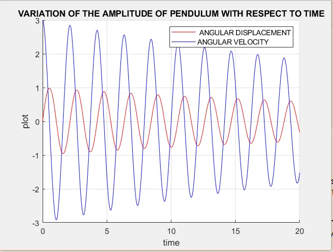
Figure 4 : The variance of angular displacement and angular velocity with respect to time

To understand the properties of the pendulum oscillation varies with the mass and damping coeffecient lets get more deeper into this cocept . Damping is basically a factor which decides the time take for the pendulum to come into rest or we can even say it as the motion undergone by the pendulum before it comes into equilibirium. ( ie the no of oscillation the pendulum takes to come back to the equilibirium) . There are three types of damping : under damped system , critically damped system , over damped system lets understand the concept more significantly :

UNDER DAMPED SYSTEM (b=0.005) m=0.1 kg	CRITICALLY DAMPED SYSTEM (b= 0.05) m = 0.1 kg	OVER DAMPED SYSTEM (b= 0.5) m = 0.1 kg
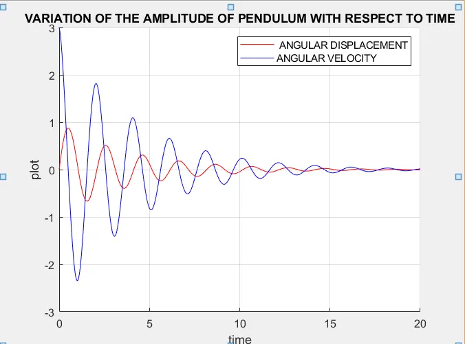Figure 5: under damped system	Figure 6 : Critically damped system	Figure 7 : Over damped system
1. From figure 5 we can see that the angular velocity and angular displacement gradually reduces with the oscillations 2. The amplitude is constant and decreases slowly with the iterations with respect to time . 3. The real time example of this concept is a car driving over a speed braker , it bumps continuously and comes back to equilibirium slowly , the shock absorber does this job . 4. damping basically reduces the damage caused to the system. 5. More vibrations	1.From figure 6 we can see that the angular displacement and angular velocity in a greater interval with respect to figure 1. 2. The no of oscillations are reduced compared to under damped system . 3. The no of oscillations taken by the system before comming to equilibirium is reduced 4. Less vibrations 5. This type of systems are generally the tuned schock absorbing reduces in which there is less vibration .	1. From the figure 7 we can see that the angular displacement and angular velocity rises with a peek and drops down slowly. 2. This system is basically very tight 3. Generally there are no oscillations . 4. This system basically doesnt have any spring or shock absorber . 5. This system generally causes damage to the body

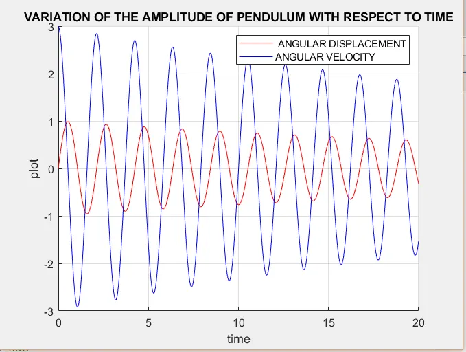
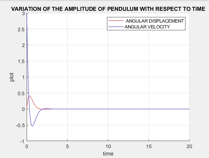
From the figure 4,5,6 ,7 and the animation video we can see clearly that how the oscillation , frequency of the pendulum is affected with respect to the mass of the pendulum bob and the damping co-effecient , from this we can conclude that the

1. When the damping co-effecient and the time span is constant the frequency or the no of oscillations is directly propotional to the mass of the pendulum.

2. When mass and the time period of the pendulum is constant the no.of oscillations or frequency of the pendulum is inversely propotional to the damping co-effecient (b).

The animation of the pendulum is attached in the youtube link given below :

https://www.youtube.com/watch?v=wfb0aH-ToWQ&feature=youtu.be