Curve fitting

AIM : To code a program to plot for the linear and cubic polynomial which is a best fit for the cp data and to find out the catogaries to classify the error criterias and determine the goodness of fit .

INTRODUCTION :

Curve fit in simple words can be explained as the best fit for a given data which can be with a degree of 2 , 3 or higher. curve fitting in simple words can be explained as an mathematical process which is used to explain ot predict some natural events. A curve fit basically construct a set of mathematical sets which is used to predict a model . Lets take an situation as an example we have a particular historical data set which has the agricultral growth represented with respect to time and we have to model a data set which fits into the histortical data with a minimum error , this can be used to decide or generate a proper plan. So if we have to find or justify that the fit modelled is the best fit this can be done flowwing some methods such as :

1. The sum of squares due to errors (SSE)
2. R- Square
3. Adjusted R- square
4. Root mean squared error ( RMSE)

A curve fit basically looks as in the figure 1 . as we can se the one is the data set and the other is the precdited data set , in simple terms an error can be defined as the difference of the predicted data set and the normal or the existing data set . A set which has a larger error can be declared as the bad fit and the set with a minimum error can be defined as the good fit this can be explained clearly from the figure 1 .

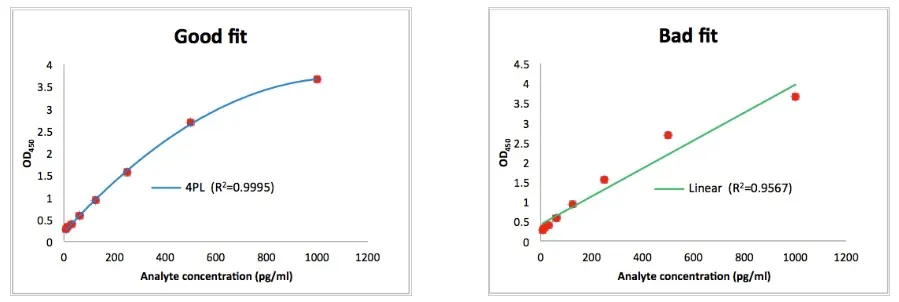
Figure 1 : good fit and the bad fit

In oder to find the best bit we are using the r square method which can be explained as follows

R- square method :

In simple words R- square method can be explained as a method or study used to determine the goodness of the fit this method basically works under the principle of corellation betwwen the predicted values and the actual values . lets look at the math behind this method in oder to find out the best fit we have to follow certain steps to evaluate the `R^2` which is an exponential value which is used to determine the goodness of fit .

SSR = `sum ( data _ (predctied)- Mean) ^ 2`

SSR is the sum of the squares of the regression which is basically the summation of the square of the difference of the predicted data set to the mean of the actual data set .

SSE = `sum ( Data _(predicted) - Data _ (actual) )^ 2`

SSE sum of squared errors can be defined as the total deviation of the respose values from the fit in simple words can be also said as the sum of the squared residuals.

SST is also called as the sum of the squares about the mean which can be also said as SST = SSR + SSE

`R^2 = (SSR)/(SST` OR `1 - (SSE)/(SST)`

The value of the R- square determines the go0odness of the fit which is as determined

0 worst possible fit

1 Best possible fit

Limitations of the r - square method :

There are few problems with the r- square method , the main one is that we cant find out that the model is biased or not lets see the other two problems

1. R- square increases every time an independent variable is added to the system or model , R-square value is never decreases , evn when it is a chance of just a corellation between the variables. A regression model containing more independent variables are generally said to be a good fit .
2. when a model consists of a exessive number of independant variables , the model becomes overly coustoumized to fit the pecularities and random noise in the sample rather then reflecting the entire population . Mathematiscians and staticians cal this type of model as over fitted model , though this have a high R-squared value the model has a decreased level of acute precission.

Lets discuss about the other few models which are also used to find the goodness of the curve fit

Adjusted R- square method :

This method is generally used to check the goodness of fit when different number of independent variables are used .

Predicted R-square method :

The proccedure for predicted R-square method can be given as :

1. first removes the data points from datasets
2. Calculate the regression equation
3. Evaluates how well the model predicts the missing information
4. Repeats this for data points in the data set

Standard error of regression :

The standard error of the regression (s) also known as the standard error of the estimate ,represents the average distance that the observed values fall from the regression line . Conveniently, it tells you how wrong the regression model is on average using the units of the response variables.

MATLAB PROGRAM :

AIM : To fit a curve to the plot of the variation of the co-effecient of pressure with respect to the temperature and do determine the goodness of the fit and also to find a method for plotting and fitting a curve exactly and accuarately.

Proccedure :

In oder to fit an accurate and preccised curve to the model of the plot " the variation of c_p of oxygen with the temperature . In oder to achieve this we can divide the program in to three sections

1. load the data and the plot variation curve and code to fit a data into the model
2. Now find out the goodnes of the fit using the R- square method
3. Now code proper curve fit using the split-wise method

Split-wise method :

There are several ways to obtain a goood fit one of the easiest method to obtain a good fit is to increase the degree of the polynomial but using this method we get a error saying that the curve is badly conditioned to avoid this we are splitting the entire curve into a certain number of segments each segment has a different value for oder of the polynomial and finally we combine all the predicted data to get a perfect fit for the curve

Steps for the program :

1. Load the data set for the variation of c_p of oxygen with respect to temperature .
2. plot the graph for the data set
3. using the polyfit command get the coeffecients for the equation to get the predicted values for the model
4. using the poly val command find the predicted values for the coeffecients which u get using the polyfit command
5. now plot the predicted model and the actual model for linear and cubic polynomial using the plot commands and the hold on command
6. use the x-label and y-label and then distinguish the plots using the legend command
7. Now find the goodness of the fit using r square method
8. now agan repeat the same proccedure from steps 1- 6 for the splitwise method but the onlydifference is here we will use this poly fit and poly val command for a n number of times cause we are dividing the model into "n" number of segments and also we are finding the coeffecients and predicted value for this "n" number of segments and then we are combining it to get the curve fit for the model
9. In this project we are finding the curve fit for the linear and cubic polynomial
10. Now again using the r-sqare method we are finding the goodness of the fit

Code :

%  Program 1 : curve fit using genral method 
close all 
clear all
clc
% loading the data set to the matlab 
% assigning the data set to temperature and cp 
cp_data = load ('data');
temperature = cp_data(:,1); % temperature column 
cp = cp_data(:,2 );   % specifc heat column
% curve fit 
% for linear or 1 st degree polynomial 
% equation = a*t+b 
coeff_1= polyfit(temperature,cp,1);
predicted_cp_1 = polyval( coeff_1,temperature);
% Now determining the coeffecients and the predicted values for third degree polynomial
% equation = at^3 + bt^2 + ct+ d 
% there are four coeffecients 
coeff_2 = polyfit(temperature,cp,3);
predicted_cp_2 = polyval(coeff_2,temperature);
% curve fit comparission of the first degree polynomial with the original data
figure(1)
hold on 
plot( temperature,cp,'linewidth',3,'color','b')
plot( temperature,predicted_cp_1,'linewidth',3,'color','r')
xlabel('temperature[k]')
ylabel('specific heat')
legend('original dataset','curve fit')
title('First degree polynomial')
grid on 

% curve fit comparission of the third degree polynomial with the original data
figure(2)
hold on 
plot( temperature,cp,'linewidth',3,'color','b')
plot( temperature,predicted_cp_2,'linewidth',3,'color','r')
xlabel('temperature[k]')
ylabel('specific heat')
legend('original dataset','curve fit')
title(' Third degree polynomial')
grid on 
% now we have to find out the goodness of the fit 
% calculating sse,ssr, sst, rmse 
error_1 = predicted_cp_1 - cp ;
error_2 = predicted_cp_2 - cp ;
n = length(cp);
i1 = 2 ;
i2 = 3 ;
% mean 
M = mean(cp);
% calculate SSE for first degree of polynomial
sse_1 = (error_1).^2;
sse_2 = (error_2).^2;
SSE_1 = sum(sse_1)
SSE_2 = sum(sse_2)
% calculating the SSR for 1 st degree and 3rd degree polynomial 
ssr_1 = ( predicted_cp_1 - M).^2;
ssr_2 = ( predicted_cp_2 - M).^2 ;
SSR_1 = sum(ssr_1)
SSR_2 = sum(ssr_2)
% calculating the SST for 1 st and 3 rd degree polynomial 
SST_1 = SSR_1 + SSE_1 
SST_2 = SSR_2 + SSE_2 
% calculating R_sq for 1 st and 3 rd degree polynomial 
R_sq_1 = SSR_1/SST_1
R_sq_2 = SSR_2/SST_2
% calculating the r_sq_adjusted for 1st and 3 rd degree polynomial
R_sq_adj_1 = 1- (((1-R_sq_1)*(n-1))/(n-i1-1))
R_sq_adj_2 = 1- (((1-R_sq_2)*(n-1))/(n-i2-1))
% calculating rmse for 1 st and 3 rd degree polynomial 
% RMSE = Root mean square error 
RMSE_1 = (SSE_1/n)^0.5
RMSE_2 = (SSE_2/n)^0.5

Figure 2 : code for finding out the curve fit for linear and cubic polynomial using general method

%  program 2 : curve fit using split wise polynomial 
 clear all 
 close all 
 clc
 % loading the data set to the matlab 
% assigning the data set to temperature and cp 
cp_data = load ('data');
temperature = cp_data(:,1); % temperature column 
cp = cp_data(:,2 );   % specifc heat column
% curve fit 
% for linear or 1 st degree polynomial 
% equation = a*t+b 
% curve fit for first degree polynomial ( dividng into five segments )
linear_coeff_1 = polyfit(temperature(1:640),cp(1:640),1);
linear_coeff_2 = polyfit(temperature(641:1280),cp(641:1280),1);
cubic_coeff_3 = polyfit(temperature(1281:1920),cp(1281:1920),1);
cubic_coeff_4 = polyfit(temperature(1921:2560),cp(1921:2560),1);
cubic_coeff_5 = polyfit(temperature(2561:3200),cp(2561:3200),1);

cubic_predicted_cp_1 = polyval(linear_coeff_1,temperature(1:640));
cubic_predicted_cp_2 = polyval(linear_coeff_2,temperature(641:1280));
cubic_predicted_cp_3 = polyval(cubic_coeff_3,temperature(1281:1920));
cubic_predicted_cp_4 = polyval(cubic_coeff_4,temperature(1921:2560));
cubic_predicted_cp_5 = polyval(cubic_coeff_5,temperature(2561:3200));

linear_predicted_cp = [cubic_predicted_cp_1;cubic_predicted_cp_2;cubic_predicted_cp_3;cubic_predicted_cp_4;cubic_predicted_cp_5];
% Now determining the coeffecients and the predicted values for third degree polynomial
% equation = at^3 + bt^2 + ct+ d 

cubic_coeff_1 = polyfit(temperature(1:640),cp(1:640),1);
cubic_coeff_2 = polyfit(temperature(641:1280),cp(641:1280),1);
cubic_coeff_3 = polyfit(temperature(1281:1920),cp(1281:1920),1);
cubic_coeff_4 = polyfit(temperature(1921:2560),cp(1921:2560),1);
cubic_coeff_5 = polyfit(temperature(2561:3200),cp(2561:3200),1);

cubic_predicted_cp_1 = polyval(cubic_coeff_1,temperature(1:640));
cubic_predicted_cp_2 = polyval(cubic_coeff_2,temperature(641:1280));
cubic_predicted_cp_3 = polyval(cubic_coeff_3,temperature(1281:1920));
cubic_predicted_cp_4 = polyval(cubic_coeff_4,temperature(1921:2560));
cubic_predicted_cp_5 = polyval(cubic_coeff_5,temperature(2561:3200));

cubic_predicted_cp = [cubic_predicted_cp_1;cubic_predicted_cp_2;cubic_predicted_cp_3;cubic_predicted_cp_4;cubic_predicted_cp_5];
% curve fit comparission of the first degree polynomial with the original data
figure(1)
hold on 
plot( temperature,cp,'linewidth',3,'color','b')
plot( temperature,linear_predicted_cp,'linewidth',3,'color','r')
xlabel('temperature[k]')
ylabel('specific heat')
legend('original dataset','curve fit')
title('First degree polynomial')
grid on 

% curve fit comparission of the third degree polynomial with the original data
figure(2)
hold on 
plot( temperature,cp,'linewidth',3,'color','b')
plot( temperature,cubic_predicted_cp,'linewidth',3,'color','r')
xlabel('temperature[k]')
ylabel('specific heat')
legend('original dataset','curve fit')
title(' Third degree polynomial')
grid on 

% now we have to find out the goodness of the fit 
% calculating sse,ssr, sst, rmse 
error_1 = linear_predicted_cp - cp ;
error_2 = cubic_predicted_cp - cp ;
n = length(cp);
i1 = 2 ;
i2 = 3 ;
% mean 
M = mean(cp);
% calculate SSE for first degree of polynomial
sse_1 = (error_1).^2;
sse_2 = (error_2).^2;
SSE_1 = sum(sse_1)
SSE_2 = sum(sse_2)
% calculating the SSR for 1 st degree and 3rd degree polynomial 
ssr_1 = ( linear_predicted_cp - M).^2;
ssr_2 = ( cubic_predicted_cp - M).^2 ;
SSR_1 = sum(ssr_1)
SSR_2 = sum(ssr_2)
% calculating the SST for 1 st and 3 rd degree polynomial 
SST_1 = SSR_1 + SSE_1 
SST_2 = SSR_2 + SSE_2 
% calculating R_sq for 1 st and 3 rd degree polynomial 
R_sq_1 = SSR_1/SST_1
R_sq_2 = SSR_2/SST_2
% calculating the r_sq_adjusted for 1st and 3 rd degree polynomial
R_sq_adj_1 = 1- (((1-R_sq_1)*(n-1))/(n-i1-1))
R_sq_adj_2 = 1- (((1-R_sq_2)*(n-1))/(n-i2-1))
% calculating rmse for 1 st and 3 rd degree polynomial 
% RMSE = Root mean square error 
RMSE_1 = (SSE_1/n)^0.5
RMSE_2 = (SSE_2/n)^0.5

Figure 3: code to find and plot the curve fit using the split wise method

RESULTS AND DISCUSSION

Program 1 :

The program 1 is the genral code to find out the predicted values and plot the comparison between the actual data set and the predicted data set we can see the comparission graph for the linear and cubic polynomial as shown in the Figure 4 and Figure five respectively. we can see the goodness of the fit also calculated using the four different methods in Figure 6. This criteria can be verified using the curve fit tool box, the output is as shown in Figure 7 and Figure 8 for linear and cubic polynomial respectively.

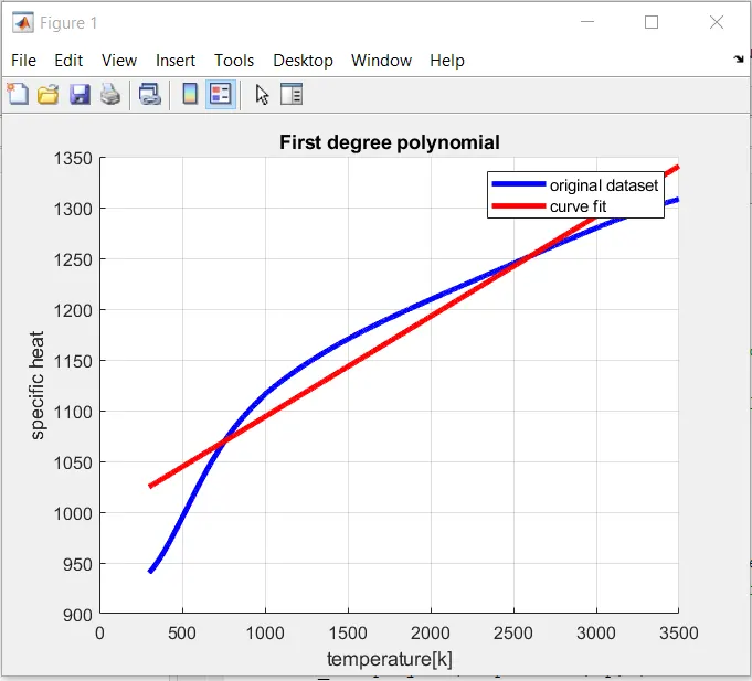
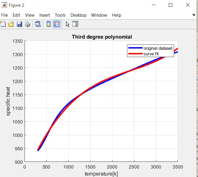
Figure 4 : first degree polynomial Figure 5 : 3 rd degree polynomial

SSE_1 =

   2.1630e+06


SSE_2 =

   9.4272e+04


SSR_1 =

   2.6631e+07


SSR_2 =

   2.8699e+07


SST_1 =

   2.8794e+07


SST_2 =

   2.8794e+07


R_sq_1 =

    0.9249


R_sq_2 =

    0.9967


R_sq_adj_1 =

    0.9248


R_sq_adj_2 =

    0.9967


RMSE_1 =

   25.9991


RMSE_2 =

    5.4277

>> 

Figure 6 : Out put for goodness of the fit using r_square , r_adjusted _square, RMSE method

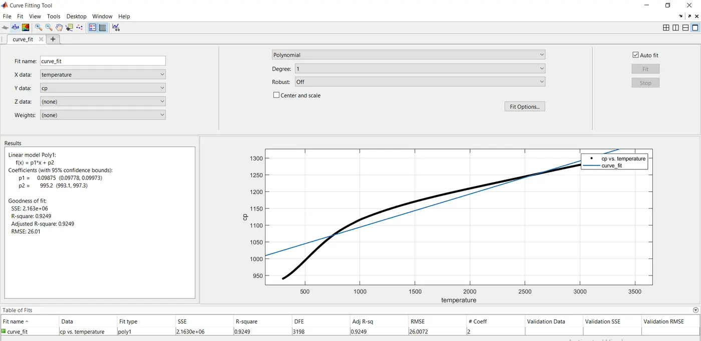
Figure 7 : Verifiying first degree polynomial using curve fit tool box

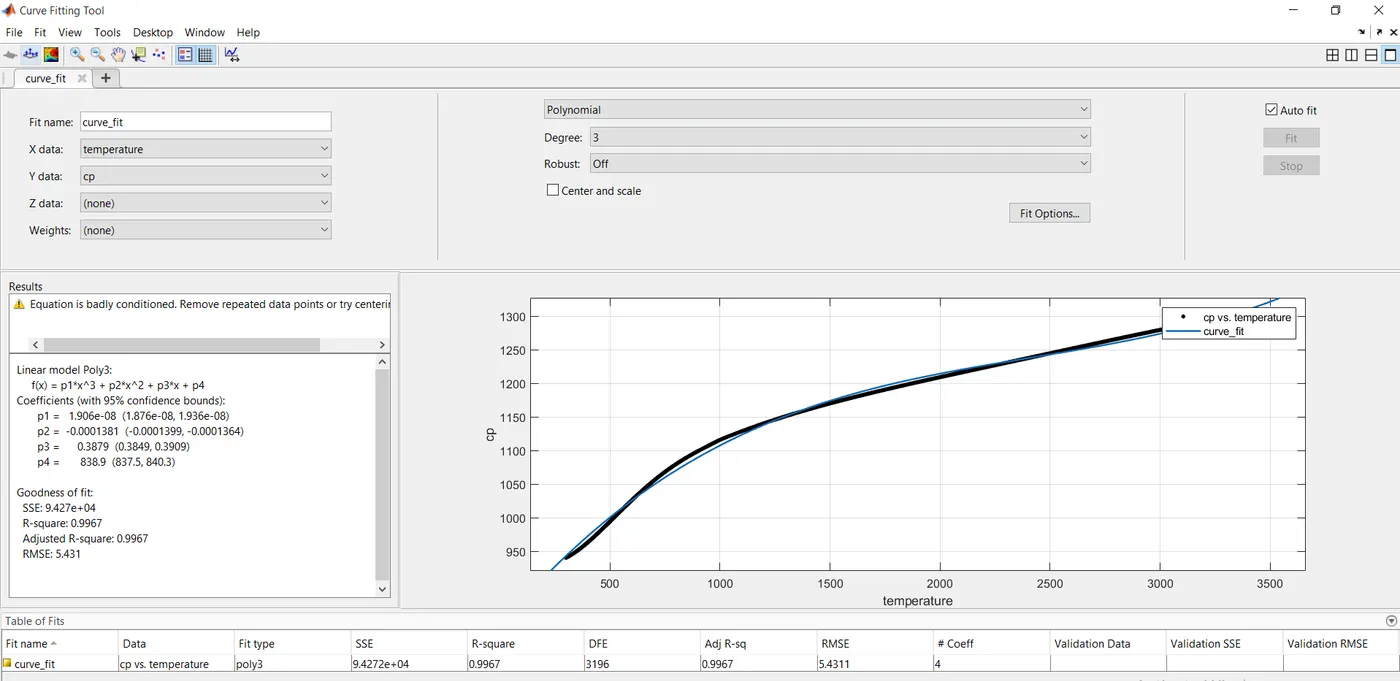
Figure 8 : Verifiying 3rd degree polynomial using curve fit tool box

from Figure 3 and Figure 6 we can say that using a higher oder degree we are getting a good fit but from Figure 8 it is seen that we are getting an error as " equation badly conditioned". This means that we are getting a good curve fit but the values are not more accurate. For rectifying this we are using the splitwise method in the program 2

Program 2 :

we are divide the whole data set into 5 segments for ploting a good curve fit , the results of this program are comparission of the original data set with the predicted data set of the linear and cubic polynomial respectively as shown in the figure 9 and Figure 10 . Now by conducting the test for the goodness of the fit as shown in Figure 11 , we can conclude that we are not getting the error as " badly conditioned equation" and we are getting a good and perfect curve fit with accurate values.

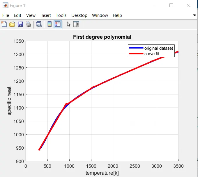
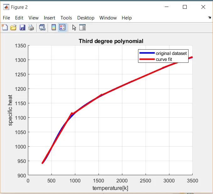
Figure 9 : split wise method using linear polynomial Figure 10 : split wise method using cubic polynomial

SSE_1 =

   1.1708e+04


SSE_2 =

   1.1708e+04


SSR_1 =

   2.8782e+07


SSR_2 =

   2.8782e+07


SST_1 =

   2.8794e+07


SST_2 =

   2.8794e+07


R_sq_1 =

    0.9996


R_sq_2 =

    0.9996


R_sq_adj_1 =

    0.9996


R_sq_adj_2 =

    0.9996


RMSE_1 =

    1.9128


RMSE_2 =

    1.9128

>> 

Figure 11 : Results for goodness of the fit using r_square , r_adjusted _square, RMSE method for split wise method