Week 7 - Simulation of a 1D Super-sonic nozzle flow simulation using Macormack Method
Here we are computing Distribution of temperature , velocity , Density, and mass flow rates in quasi 1D isentropic subsonic and super sonic flows using two forms of governing solutions by MacCormack's technique. The two forms of governing equations are
1. Non conservative technique
2. Conservative technique
First we will solve the using Non Conservative form of Governing equations
Lets write the Governing equations in Non conservative form
Continuity Equation
`(delrho)/(delt) = -rho*((delv)/(delt))-rho*v*((dellnA)/(delx))-v*((delrho)/(delx))`
Momentum Equation
`(delv)/(delt) = -v*(delv)/(delx)- (1/gamma)*((delt)/(delt)+(t/rho)*(delrho)/(delx))`
Energy Equation
`(delt)/(delt) = -v*(delt)/(delx)-(gamma-1)*t*((delv)/(delx)+v*(del(lna))/(delx))`
The above equations are written in Non dimensional form
Now lets take initial conditions of the flow
`rho = 1-0.3146*x`
`t = 1-0.2314*x`
`v = (0.1+1.09*x)*sqrtt`
Now we will write code in matlab to see how the variables are changing at different times and different locations
Matlab function code for Non conservative method
function [ rho , v, t ,m , rho_th , v_th, t_th ,m_th] = nonconservative( x , dx ,n, gamma)

%Initial flow conditions

rho = 1-0.3146*x ;

t = 1-0.2341*x ;

v = (0.1+1.09*x).*t.^0.5 ;

a = 1+ 2.2*(x-1.5).^2;

% Time steps

nt = 1000;


%Time loop starts

for k = 1:nt

    rhoold = rho ;
    vold = v;
    told = t;

    c = 0.5 ;

    for i = 1:n
        p(i) = c*(dx/(sqrt(t(i))+v(i))) ;

    end

    dt = min(p) ;

    % Predictor method starts


    for j = 2:n-1


        dvdx = (v(j+1)-v(j))/dx ;
        drhodx = (rho(j+1)-rho(j))/dx;
        dtdx = (t(j+1)-t(j))/dx ;
        dlogadx = (log(a(j+1))-log(a(j)))/dx;

         % continuity equation

        drhodt_p(j) = -rho(j)*dvdx-rho(j)*v(j)*dlogadx-v(j)*drhodx ;

        %momentum equation

        dvdt_p(j) = -v(j)*dvdx-(1/gamma)*((dtdx+t(j)/rho(j))*drhodx);

        % Energy equation

        dtdt_p(j) = -v(j)*dtdx - (gamma-1)*t(j)*(dvdx+v(j)*dlogadx);

        %solution update

        rho(j) = rho(j) + drhodt_p(j)*dt;
        v(j) = v(j) + dvdt_p(j)*dt;
        t(j) = t(j) + dtdt_p(j)*dt;
     end
    % prdectior step ends

    %corrector step starts

    for j = 2:n-1


        dvdx = (v(j)-v(j-1))/dx ;
        drhodx = (rho(j)-rho(j-1))/dx;
        dtdx = (t(j)-t(j-1))/dx ;
        dlogadx = (log(a(j))-log(a(j-1)))/dx;

         % continuity equation

        drhodt_c(j) = -rho(j)*dvdx-rho(j)*v(j)*dlogadx-v(j)*drhodx ;

        %momentum equation

        dvdt_c(j) = -v(j)*dvdx-(1/gamma)*((dtdx+t(j)/rho(j))*drhodx);

        % Energy equation

        dtdt_c(j) = -v(j)*dtdx - (gamma-1)*t(j)*(dvdx+v(j)*dlogadx);

        %solution update

        rho(j) = rho(j) + drhodt_c(j)*dt;
        v(j) = v(j) + dvdt_c(j)*dt;
        t(j) = t(j) + dtdt_c(j)*dt;
    end

    %compute the average time derivatives

    drhodt  = 0.5*( drhodt_p+ drhodt_c);

    dvdt = 0.5*(dvdt_p + dvdt_c);

    dtdt = 0.5*(dtdt_p + dtdt_c);

    % Final solution
   for i = 2:n-1

    rho(i) = rhoold(i) + drhodt(i)*dt;

    v(i) = vold(i)+ dvdt(i)*dt;

    t(i) = told(i) + dtdt(i)*dt;

   end

   %Apply intial conditions
   %Inlet

   rho(1) = 1;

   t(1) = 1 ;

   v(1) = 2*v(2)-v(3);

   %outlet

   v(n) = 2*v(n-1)-v(n-2);

   rho(n) = 2*rho(n-1)-rho(n-2);

   t(n) = 2*t(n-1) - t(n-2);


   for i = 1:n

       m(i) = rho(i)*a(i)*v(i);

   end

   %Comparision for convergence at throat

   rho_th(k) = rho(16);

   v_th(k) = v(16);

   t_th(k) = t(16) ;

   m_th(k) = m(16) ;


   %Plotting
   figure(2)
   subplot(2,2,1)
   plot(x,rho)
   xlabel('x')
   ylabel('Density')
   subplot(2,2,2)
   plot(x,t)
   xlabel('x')
   ylabel('Temperature')
   subplot(2,2,3)
   plot(x,v)
   xlabel('x')
   ylabel('Velocity')
   subplot(2,2,4)
   plot(x,v)
   xlabel('x')
   ylabel('Mass flow')


 end
Now we will write the equations for Conservative method and we will write the function code for the Conservative method
Lets write the Governing equations in Conservative form
Continuty equation
`(del(rho*a))/dt+(del(rho*a*v))/dx = 0`--------- eq -1
Momentum equation
`(del(rho*a*v))/(delt)+(del(rho*a*v^2)+(1/gamma)*P*a)/dx = (1/gamma)*P*(dela)/(delx)` ---------- eq -2
Energy equations
`(del(rho*(e/(gamma-1))+(gamma/2)*v^2)*a)/dt +( del(rho*(e/(gamma-1)+(gamma/2)*v^2)*v*a+rho*a*v))/(dx) =0` -------------eq-3
The above equatiuons are non dimensional equations
lets convert the above equations into generic form by introducing new variables so that we can write code and get the distributions of the variables
`u1 = rho*a` -------------- eq-4
`u2 = rho*v*a` -------------- eq-5
`u3 = u1*((t/(gamma-1))+(gamma/2)*v^2)`----------- eq-6
`f1 = rho*a*v` ------------------------------ eq-7
`f2 = rho*a*v+ (1/gamma)*P*a` ------------------------ eq-8
`f3 = rho*((e/(gamma-1))+(gamma/2)*v^2)*v*a+P*a*v` -------------------- eq-9
`j2 = (gamma-1)/gamma*(u3-(gamma/2)*(u2^2)/(u1^2)*(del(lna))/dx)` eq-10
Now lets write the equations for e (energy) in terms of t (temperature) and P(pressure) in terms of density and temperature
`e = R*t/(gamma-1)` ----- eq 11
`P = rho*t` --------- eq12
Now by using eq 12 we will convert f2 in terms of u1,u2,u3
`f2 = (u2^2)/(u1)+(gamma-1)/(gamma)*(u3-(gamma/2)*((u2^2)/(u1)))`
Now will use eq-4 and eq12 we will write f3 in terms of u1,u2,u3
`f3 = (gamma)*(u2*u3)/(u1)-(gamma-1)*(gamma/2)*((u2^3)/(u1^2))`
and by loking the equations 7 and 5
f1 = u2
By solving the above equations and continuity , momentum , and energy equations we will get the following deriavative equaitons
`(delu1)/dt = -(delf1)/dx`
`(delu2)/(delt) = -(delf2)/dx+j2`
`(delu3)/(delx) = -(delf3)/(delx)`
By using the above equations we will write the code and get the distribution
lets take initial conditions
1. `0<=x<0.5`
`rho =1`
`t =1`
2. `0.5<=x<=1.5`
`rho = 1-0.366*(x-0.5)`
`t = 1-0.167*(x-0.5)`
3. `1.5
`rho =0.634-0.3879*(x-1.5)`
`t = 0.833-0.3507*(x-1.5)`
Now lets write the matlab function code for conservative method
function [ rho , v ,t , m ,rho_th,v_th,t_th,m_th ] = conservative(x,dx,n,gamma)

a = 1+ 2.2*(x-1.5).^2;

for i = 1:n

    if x(i)>=0 && x(i)<0.5

       rho(i) = 1;
       t(i) = 1;

    elseif x(i)>= 0.5 && x(i)<1.5

        rho(i) = 1-0.366*(x(i)-0.5) ;
        t(i)  = 1- 0.167*(x(i)-0.5) ;

    elseif x(i)>=1.5 && x(i)<=3

        rho(i) = 0.634-0.3879*(x(i)-1.5) ;
        t(i)  = 0.833-0.3507*(x(i)-1.5) ;
    end

    v(i) = 0.59/(rho(i)*a(i))  ;

end


%giving the values for U1,U2,U3

for i = 1 : n

    u1(i) = rho(i)*a(i) ;

    u2(i) = rho(i)*a(i)*v(i) ;

    u3(i) = u1(i)*(t(i)/(gamma-1) + (gamma/2)*v(i)^2) ;

end

nt = 1000 ;

for k = 1:nt

u1old = u1;

u2old = u2;

u3old = u3;

c = 0.5 ;

for i = 1:n

p(i) = c*(dx/(sqrt(t(i))+v(i)));

end

dt = min(p);

%lets calculate f1,f2,f3

for i = 1:n

    f1(i) = u2(i) ;

    f2(i)  = (u2(i)^2/u1(i))  + ((gamma-1)/gamma)*(u3(i)- (gamma/2)*(u2(i)^2/u1(i))) ;

    f3(i)  = gamma*(u2(i)*u3(i)/u1(i)) - (gamma*(gamma-1)/2)*(u2(i)^3/u1(i)^2) ;

end

% lets start predictor step

for i = 2:n-1

    dadx = (a(i+1)-a(i))/dx ;

    j2(i) = (1/gamma)*rho(i)*t(i)*dadx;

    du1dt_p(i) = - (f1(i+1)-f1(i))/dx ;

    du2dt_p(i)  = - (f2(i+1)-f2(i))/dx + j2(i) ;

    du3dt_p(i)  = -(f3(i+1)-f3(i))/dx ;

    u1(i) = u1(i) + du1dt_p(i)*dt ;

    u2(i)  = u2(i) + du2dt_p(i)*dt ;

    u3(i)  = u3(i) + du3dt_p(i)*dt;

    rho(i) = u1(i)/a(i) ;

    v(i) = u2(i)/u1(i) ;

    t(i)  = (gamma-1)*((u3(i)/u1(i))-(gamma/2)*v(i)^2) ;

end

% after the predictor step lets do corrector step

%update the values for f1,f2,f3


for i = 1:n

    f1(i) = u2(i) ;

    f2(i)  = ((u2(i)^2)/u1(i))  + ((gamma-1)/gamma)*(u3(i)- (gamma/2)*(u2(i)^2/u1(i))) ;

    f3(i)  = gamma*((u2(i)*u3(i))/u1(i)) - (gamma*(gamma-1)/2)*(u2(i)^3/u1(i)^2) ;

end

for i = 2:n-1

    dadx = (a(i)-a(i-1))/dx ;

    j2(i) = (1/gamma)*rho(i)*t(i)*dadx ;

    du1dt_c(i) = - (f1(i)-f1(i-1))/dx ;

    du2dt_c(i) = - (f2(i)-f2(i-1))/dx + j2(i) ;

    du3dt_c(i) = - (f3(i)-f3(i-1))/dx ;

end

for i = 2:n-1

    du1dt(i) = 0.5*(du1dt_p(i)+du1dt_c(i)) ;

    du2dt(i) = 0.5*(du2dt_p(i)+du2dt_c(i));

    du3dt(i) = 0.5*(du3dt_p(i)+du3dt_c(i));

end

%lets update the values

for i = 2:n-1

    u1(i) = u1old(i)+ du1dt(i)*dt ;

    u2(i) = u2old(i) + du2dt(i)*dt ;

    u3(i) = u3old(i) + du3dt(i)*dt;

    rho(i) = u1(i)/a(i) ;

    v(i) = u2(i)/u1(i) ;

    t(i) = (gamma-1)*((u3(i)/u1(i)) - (gamma/2)*v(i)^2) ;


end

%inlet conditions

u1(1) = a(1);

u2(1) = 2*u2(2)-u2(3) ;

v(1) = u2(1)/u1(1) ;

t(1) = 1;

u3(1) = u1(1)*(t(1)/(gamma-1) - (gamma/2)*(v(1)^2)) ;

%outlet conditions

u1(n) = 2*u1(n-1)-u1(n-2);

u2(n) = 2*u2(n-1)-u2(n-2) ;

u3(n) = 2*u3(n-1)-u3(n-2) ;

rho(n) = u1(n)/a(n) ;

v(n) = u2(n)/u1(n) ;

t(n) = (gamma-1)*((u3(n)/u1(n))- 0.5*gamma*(v(n)^2)) ;

for i = 1 : n

    m(i) = rho(i)*a(i)*v(i);

end

  %Comparision for convergence at throat

   rho_th(k) = rho(16);

   v_th(k) = v(16);

   t_th(k) = t(16) ;

   m_th(k) = m(16) ;

 %Plotting
   figure(1)
   subplot(2,2,1)
   plot(x,rho)
   xlabel('x')
   ylabel('Density')
   subplot(2,2,2)
   plot(x,t)
   xlabel('x')
   ylabel('Temperature')
   subplot(2,2,3)
   plot(x,v)
   xlabel('x')
   ylabel('Velocity')
   subplot(2,2,4)
   plot(x,m)
   xlabel('x')
   ylabel('Mass flow ')


end
Now lets write the main code and compare the two form of methods
clear all
close all
clc

n = 31 ;

x = linspace(0,3,n) ;

dx = x(2)-x(1) ;

gamma = 1.4 ;


[ rho1, v1 , t1,m1,rho1_th,v1_th,t1_th,m1_th] = conservative(x,dx,n,gamma) ;

[rho2 , v2,t2, m2,rho2_th,v2_th,t2_th,m2_th]  = nonconservative(x,dx,n,gamma) ;

k = linspace(1,1000,1000) ;

% Comparison of mass flow rates

figure(3)
plot(x,m1)
hold on
plot(x,m2)
xlabel('x')
ylabel('Mass flow rates')
legend('conservative','nonconservative')

figure(4)
subplot(2,2,1)
plot(k,rho1_th)
hold on
plot(k,rho2_th)
xlabel('time step')
ylabel('Density variation')
subplot(2,2,2)
plot(k,v1_th)
hold on
plot(k,v2_th)
xlabel('Time step')
ylabel('Velocity variation')
subplot(2,2,3)
plot(k,t1_th)
hold on
plot(k,t2_th)
xlabel('Time step')
ylabel('Temperature variation')
subplot(2,2,4)
plot(k,m1_th)
hold on
plot(k,m2_th)
xlabel('Time step')
ylabel('Mass variation')
Now lets plot the steady state distribution of the variables
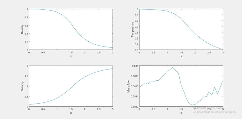
PLOTS BY CONSERVATIVE METHOD
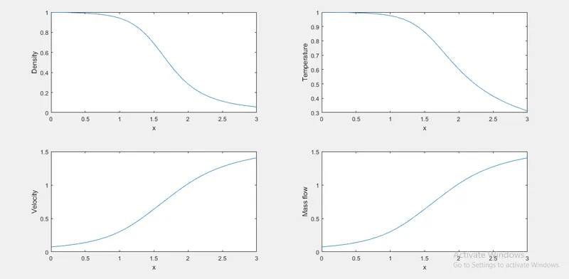
PLOTS BY NONCONSERVATIVE METHOD
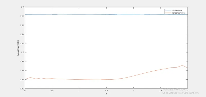
COMPARISON OF MASS FLOW RATES BY CONSERVATIVE AND NON CONSERVATIVE METHOD
NOW LETS COMPARE THE CONVERGENCE RATE OF THE BOTH THE FORMS FOR EACH VARIABLE AT PARTICULAR LACOTION i.e THROAT LOCATION
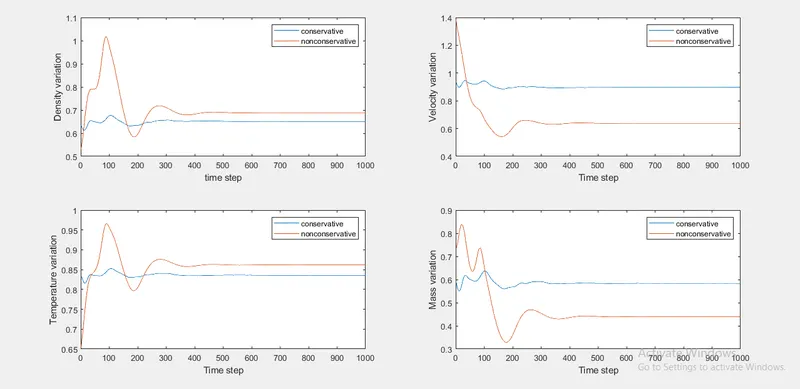
By the above plots we can say that conservative results are converging faster than non conservative
The mass flow rate calculated at different locations by using conservative method are observed to be constant