Week 5 - Mid term project - Solving the steady and unsteady 2D heat conduction problem
Matlab code for solving the above problem in steady state
clear all
close all
clc

%Inital conditions

nx1 = 10;

nx2 = 10 ;


x = linspace(0,1,nx2);
y  = linspace(0,1,nx1);

error = 9e9;
error1 = 9e9;
error2 = 9e9;

tol = 1e-4;

dx = x(2)-x(1);

dy = y(2)-y(1);

[ xx yy ] = meshgrid(x,y);


p =1;

while(p<4)


if(p==1)

%Boundary conditions

t = 300*ones(nx1,nx2);

t(1,:) = 600;
t(:,1) = 400;
t(nx1,:) = 900;
t(:,nx2) = 800;

told = t;
t_initial = t;


jacob_iter = 1;
% jacob method
%Iteration starts

while(error>tol)

    % SPACE LOOP

    for i= 2:nx1-1

        for j = 2:nx2-1

         t(i,j) = 0.5*((dx^2*dy^2)/(dx^2+dy^2))*((told(i,j+1)+told(i,j-1))/(dx^2) + (told(i+1,j)+told(i-1,j))/(dy^2)) ;

        end

    end
    error = max(max((abs(told-t))));


    %updating the old velocitites with the new velocities for the next
    %iteration

   told = t;

    jacob_iter = jacob_iter + 1;

    %Plotting

    figure(p)
    [x y] = contourf(xx,yy,t)
    colormap(jet)
    colorbar
    set(gca,'YDIR','reverse')
    pause(0.3)
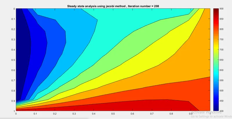
     title_text = sprintf('Steady state analysis using jacobi method , Iteration number = %d',jacob_iter);
     title(title_text)

     pause(0.3)


end
end

if(p==2)

 %Boundary conditions

t1 = 300*ones(nx1,nx2);

t1(1,:) = 600;
t1(:,1) = 400;
t1(nx1,:) = 900;
t1(:,nx2) = 800;

told1 = t1;
t_initial1 = t1;

%now lets do for gauss siedal method

t1 = t_initial1;

GS_iter = 1;

while(error1>tol)

    %Space loop starts

    for i= 2:nx1-1

        for j = 2:nx2-1

         t1(i,j) = 0.5*((dx^2*dy^2)/(dx^2+dy^2))*((t1(i,j+1)+told1(i,j-1))/(dx^2) + (t1(i+1,j)+told1(i-1,j))/(dy^2)) ;

        end

    end
    error1 = max(max(abs(told1-t1)));


    GS_iter = GS_iter + 1;

    %Plotting
    figure(p)
    [x,y] = contourf(xx,yy,t1)
    colormap(jet)
    clabel(x,y)
    set(gca,'YDIR','reverse')
    pause(0.3)
     title_text = sprintf('Steady state analysis using gauss siedal ,Iteration number = %d',GS_iter);
     title(title_text)


    % Updating the old velocities with the new velocities for the next
    % iteration
    told1 = t1;
end
end

if(p==3)
t2 = 300*ones(nx1,nx2);

t2(1,:) = 600;
t2(:,1) = 400;
t2(nx1,:) = 900;
t2(:,nx2) = 800;

told2 = t2;
t_initial2 = t2;

%Now lets do SOR method

sor_iter = 1;
alpha = 1.2;

while(error2>tol)

    %Space loop starts

    for i= 2:nx1-1

        for j = 2:nx2-1

            t2(i,j) = (1-alpha)*told2(i,j) + alpha*0.5*((dx^2*dy^2)/(dx^2+dy^2))*((told2(i,j+1)+t2(i,j-1))/(dx^2) + (told2(i+1,j)+t2(i-1,j))/(dy^2));

        end

    end

    error2 = max(max(abs(t2-told2)));

    %Updating the old velocities with the new velocities for next iteration

    told2 = t2;

    sor_iter = sor_iter + 1 ;

    %Plotting
    figure(p)
    [x,y] = contourf(xx,yy,t2)
    colormap(jet)
    clabel(x,y)
    set(gca,'YDIR','reverse')
    pause(0.3)
     title_text = sprintf('Steady state analysis using SOR method ,Iteration number = %d',sor_iter);
     title(title_text)

end
end

p = p+1;
end
Plots
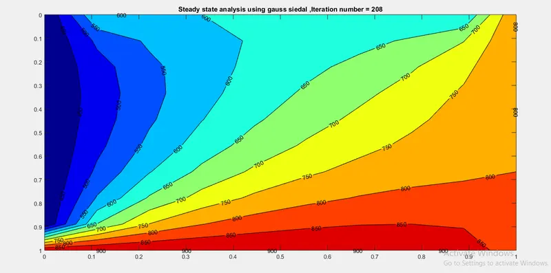
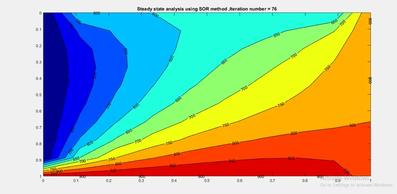
Matlab code for solving transient using explicit scheme
%Transient using Explicit method
nx = 10 ;
ny = 10;

x = linspace(0,1,nx);

y = linspace(0,1,ny);

[ xx yy ] = meshgrid(x,y);

% Boundary conditions

t = 300*ones(nx,ny);

t(1,:) = 600;
t(nx,:) = 900;
t(:,1) = 400;
t(:,ny) = 800;

t(1,1) = (600+400)/2;
t(1,ny) = (600+800)/2;
t(nx,1) = (900+400)/2;
t(nx,ny) = (900+800)/2;


dt = 0.001;
dx = x(2)-x(1) ;
dy = y(2)-y(1);

alpha = 1.4;

k1 = alpha*dt/(dx^2);
k2 = alpha*dt/(dy^2);

nt = 1600;
told = t;

%Time loop starts

for m = 1:1600

    %space loop starst

    for i = 2 : nx-1;

        for j = 2:ny-1

            term2 = k1*(told(i+1,j)-2*told(i,j)+told(i-1,j));
            term3 = k2*(told(i,j-1)-2*told(i,j)+told(i,j+1));

            t(i,j) = told(i,j)+term2+term3;

        end
    end

    told = t;

end
%Plotting

figure(1)
 [x y] = contourf(xx,yy,t)
 colormap(jet)
 colorbar
 set(gca,'YDIR','reverse')
 pause(0.03)
   title_text = sprintf('Transient heat conduction by Explicit method ');
        title(title_text);
Plots
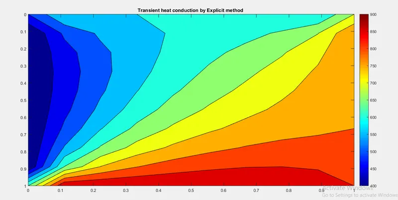
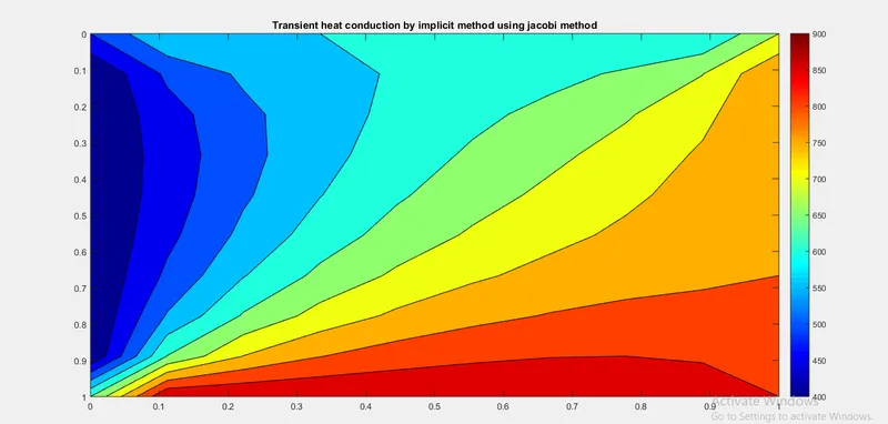
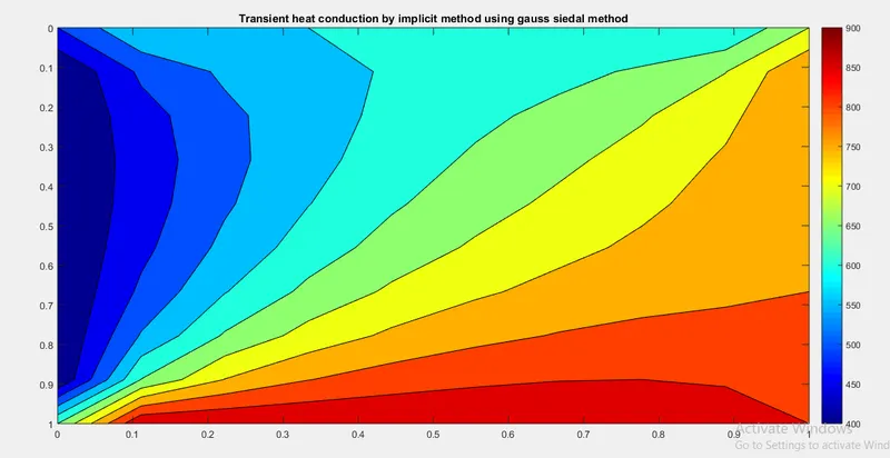
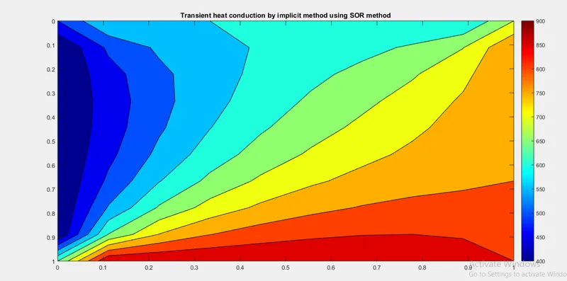
Matlab code to solve transient 2D heat conduction by implicit method
% Transient analysis using implicit scheme

% inputs

nx = 10 ;
ny = 10;

x = linspace(0,1,nx);

y = linspace(0,1,ny);

[ xx yy ] = meshgrid(x,y);

% Implicit using Jacobi method

t = 300*ones(nx,ny);

t(1,:) = 600;
t(nx,:) = 900;
t(:,1) = 400;
t(:,ny) = 800;

t(1,1) = (600+400)/2;
t(1,ny) = (600+800)/2;
t(nx,1) = (900+400)/2;
t(nx,ny) = (900+800)/2;

tol = 1e-4;

dt = 0.001;
dx = x(2)-x(1) ;
dy = y(2)-y(1);

alpha = 1.4;

k1 = alpha*dt/(dx^2);
k2 = alpha*dt/(dy^2);


jacobi_iter = 1;

told = t;

tp = t;


nt = 1600;
error = 9e9;

% time loops starts

for m = 1:nt

    term1 = 1/(1+2*k1+2*k2) ;
    term2 = k1*term1;
    term3 = k2*term1;

    error = 9e9;
    while(error>tol)

        % Space loop starts

        for i= 2:nx-1

            for j = 2:ny-1;

                H = told(i-1,j)+told(i+1,j);
                V = told(i,j-1)+told(i,j+1);

                t(i,j) = term1*tp(i,j)+term2*H + term3*V ;

            end
        end

        error = max(max(abs(told-t)));

        %Updating the old velocities with the new velocities for the next
        %iteration

        told =t;

        jacobi_iter = jacobi_iter + 1 ;


    end

    %Updating the old velocities with the new velocities for the next time
    %step

   tp = t;

end

%plotting

 figure(1)
       [x y] = contourf(xx,yy,t)
        colormap(jet)
        colorbar
        set(gca,'YDIR','reverse')
        pause(0.3)
        title_text = sprintf('Transient heat conduction by implicit method using jacobi method');
        title(title_text);

% Implicit using the Gauss jourdan method

% Boundary conditions
 t1 = 300*ones(nx,ny);

t1(1,:) = 600;
t1(nx,:) = 900;
t1(:,1) = 400;
t1(:,ny) = 800;

t1(1,1) = (600+400)/2;
t1(1,ny) = (600+800)/2;
t1(nx,1) = (900+400)/2;
t1(nx,ny) = (900+800)/2;

told1 = t1;

tp1 = t1;

error1 = 9e9;

GS_iter = 1;

% time loop starts

for m = 1:nt

     term1 = 1/(1+2*k1+2*k2) ;
    term2 = k1*term1;
    term3 = k2*term1;

    error1 = 9e9;

    %Space loop starts

    while(error1>tol)

    for i = 2:nx-1

        for j = 2:ny-1

            H = t1(i-1,j)+told1(i+1,j);
            V = t1(i,j-1)+told1(i,j+1);

             t1(i,j) = term1*tp1(i,j)+term2*H + term3*V ;

        end
    end

    error1 = max(max(abs(told1-t1)));

    % updating the old velocities with new velocities for next iteration

    told1 = t1;

    GS_iter = GS_iter + 1 ;

    end

    %Updating the old velocities with new velocities for next time step

    tp1 = t1;

end
% Plotting

figure(2)
 [x y] = contourf(xx,yy,t1)
    colormap(jet)
    colorbar
    set(gca,'YDIR','reverse')
    pause(0.3)
      title_text = sprintf('Transient heat conduction by implicit method using gauss siedal method');
        title(title_text);

%SOR method

%Boundary conditions to SOR method

 t2 = 300*ones(nx,ny);

t2(1,:) = 600;
t2(nx,:) = 900;
t2(:,1) = 400;
t2(:,ny) = 800;

t2(1,1) = (600+400)/2;
t2(1,ny) = (600+800)/2;
t2(nx,1) = (900+400)/2;
t2(nx,ny) = (900+800)/2;

told2 = t2;

tp2 = t2;

error2 = 9e9;

omega = 1.2;

sor_iter = 1;

%Time loops starts

for m = 1:nt

      term1 = 1/(1+2*k1+2*k2) ;
    term2 = k1*term1;
    term3 = k2*term1;

    error2 = 9e9;

    while(error2>tol)

        %Space loop starts

        for i= 2:nx-1;

            for j = 2:ny-1

            H = t2(i-1,j)+told2(i+1,j);
            V = t2(i,j-1)+told2(i,j+1);

             t2(i,j) = (1-omega)*(told2(i,j))+omega*(term1*tp2(i,j)+term2*H + term3*V );

            end
        end

        error2 = max(max(abs(told2-t2)));

        %Updating thr old velocities with the new velocities for next
        %iteration

        told2 = t2;

        sor_iter = sor_iter +1 ;

    end

    %updating the old velocities with new velocities for next time step

    tp2 = t2;

end

%Plotting

figure(3)
 [x y] = contourf(xx,yy,t2)
    colormap(jet)
    colorbar
    set(gca,'YDIR','reverse')
    pause(0.3)
      title_text = sprintf('Transient heat conduction by implicit method using SOR method');
        title(title_text);
Plots