Week 3 - Taylor table method and Matlab code

The matlab code

clear all
close all
clc
% matrices to solve variables for skewed right side difference
B1 = [ 1 1 1 1 1 1 ; 0 1 2 3 4 5 ; 0 1 4 9 16 25 ; 0 1 8 27 64 125 ;0 1 16 81 256 625 ; 0 1 32 243 1024 3125]

A1 = [0 ; 0;2;0;0;0]
X1 = inv(B1)*A1;
a1 = X1(1);
b1 = X1(2);
c1 = X1(3);
d1 = X1(4);
e1 = X1(5);
g1 = X1(6);
% matrices to solve variables for skewed left side difference

B2 = [ 1 1 1 1 1 1 ; 0 -1 -2 -3 -4 -5 ; 0 1 4 9 16 25 ; 0 -1 -8 -27 -64 -125 ; 0 1 16 81 256 625 ; 0 -1 -32 -243 -1024 -3125];
A2 = [ 0 ; 0 ; 2 ; 0 ; 0 ; 0 ];
X2 = inv(B2)*(A2);
a2 = X2(1);
b2 = X2(2);
c2 = X2(3);
d2 = X2(4);
e2 = X2(5);
g2 = X2(6);

% matrices to solve variables for Central differencing
B3 = [ 1 1 1 1 1  ; -2 -1 0 1 2 ; 4 1 0 1 4 ; -8 -1 0 1 8 ; 16 1 0 1 16 ];
A3 = [0 ; 0 ; 2 ; 0 ; 0 ];
X3 = inv(B3)*(A3);
a3 = X3(1);
b3 = X3(2);
c3 = X3(3);
d3 = X3(4);
e3 = X3(5);
x = pi/3;
dx = linspace(pi/4,pi/40,20);

for i = 1:length(dx)

    % numerical derivative function for skewed right sided difference

    numerical_derivative_1(i) = (a1*exp(x)*cos(x)+b1*exp(x+dx(i))*cos(x+dx(i))+c1*exp(x+2*dx(i))*cos(x+2*dx(i))+d1*exp(x+3*dx(i))*cos(x+3*dx(i))+e1*exp(x+4*dx(i))*cos(x+4*dx(i))+g1*exp(x+5*dx(i))*cos(x+5*dx(i)))/(dx(i)^2);
 
    % numerical derivative function for skewed left sided difference

    numerical_derivative_2(i) = (a2*exp(x)*cos(x)+b2*exp(x+dx(i))*cos(x+dx(i))+c2*exp(x+2*dx(i))*cos(x+2*dx(i))+d2*exp(x+3*dx(i))*cos(x+3*dx(i))+e2*exp(x+4*dx(i))*cos(x+4*dx(i))+g2*exp(x+5*dx(i))*cos(x+5*dx(i)))/(dx(i)^2);


    % numerical derivative function for Central differencing

    numerical_derivative_3(i) = (a3*exp(x-2*dx(i))*cos(x-2*dx(i))+b3*exp(x-dx(i))*cos(x-dx(i))+c3*exp(x)*cos(x)+d3*exp(x+dx(i))*cos(x+dx(i))+e3*exp(x+2*dx(i))*cos(x+2*dx(i)))/(dx(i)^2);

analytical_derivative = -2*exp(x)*sin(x);

% error of skewed right sided difference
error1(i) = abs( numerical_derivative_1(i)-analytical_derivative);

%error of skewed left sided difference
error2(i) = abs( numerical_derivative_2(i)-analytical_derivative);

%error of Central differencing
error3(i) = abs( numerical_derivative_3(i)-analytical_derivative);

end


%plotting and comparing 

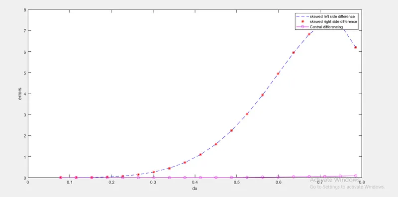
figure(1)
plot(dx,error2,'--b',dx,error1,'*r')
hold on
plot(dx,error3,'-om')

xlabel('dx')
ylabel('errors')
legend('skewed left side difference','skewed right side difference','Central differencing')

The graphs

Conclusions :

From the above conclusions the central differencing is being more accurate than the skewed right and sweked left side difference methods

1. The skewed left side and the right side uses p+q

where p is the order of the derivative and q is the order of approximation needed

p = 2 , q = 4 . Total terms required = 6 terms

2. The central differencing uses p+q-1

Total terms = 5 terms

so we have derived fourth order approximation

Some times skewed is useful and central differencing is not useful because

Skewed utilises the date either left or the right data points from the point of consideration , where as the central difference scheme uses the data both from the left and the right data points from the point of consideration . Sckewed scheme is used when the direction of the flow is known . When the method of characterisations are known for a flow using the sckewed differencing method gives the higher ordrer accuracy compared to the central differencing