Week 11 - Simulation of Flow through a pipe in OpenFoam
Hagen-Poiseullie's equation is a physical law used to calculate the pressure drop across a pipe of uniform crossection through which there is laminar flow of a viscous , incompressible, Newtonian fluid
Hagen-Poiseullies equation is
`Deltap = (32* mu*l*V_(avg))/(d^2)`
`nu = mu/rho`
`V_(avg) = (Re*mu)/(rho*d)`
`V_(max) = 2*V_(avg)`
`Deltap` is change in the pressure of across a pipe of uniform crossection because of viscosity of liquid .
`mu` is dynamic viscosity .
`V_(avg)` is average velocity of the liquid through the pipe .
`rho` = density of the liquid .
d is the diameter of the pipe .
`V_(max)` is maximum velocity
HydroDynamic length :
The hydrodynamic entrance region refers to the area of a pipe where fluid entering a pipe develops a velocity profile due to viscous forces propagating from the interior wall of a pipe. This region is characterized by a non-uniform flow. The fluid enters a pipe at a uniform velocity, then fluid particles in the layer in contact with the surface of the pipe come to a complete stop due to the no slip condition . Due to viscous forces within the fluid, the layer in contact with the pipe surface resists the motion of adjacent layers and slows adjacent layers of fluid down gradually, forming a velocity profile. For the conservation of mass to hold true, the velocity of layers of the fluid in the center of the pipe increases to compensate for the reduced velocities of the layers of fluid near the pipe surface. This develops a velocity gradient across the cross section of the pipe.
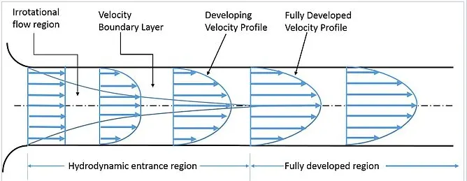
Calculating hydrodynamic length
le = 0.05*re*d
Assumptions
1.The Reynalds number is 2100 . So the flow is considered to be laminar .
2.Diameter of the pipe is 10 mm.
3.Dynamic Vsicosity `mu`= 0.00089 N/m^2.
4.Density `rho` = 997 kg/m^2.
Lets simulate a incompresible laminar flow through a pipe by OpenFoam
Lets generate blockMeshDict file from matlab so that it can be used to simulate flow through any wedge angle
Matlab code to generate blockMeshDict file to simulate incompressible laminar flow through a pipe of any wedge angle
clear all
close all
clc

% variables
re = 2100;

d = 0.015 ;

r = d/2;
mu = 0.00089 ;
theta = 5 ;
le = 0.05*re*d;
rho = 997;
nu = mu/rho ;


v_avg = (re*mu)/(rho*d) ;

v_max = 2*v_avg ;

l = le+1;

deltap = (32*mu*l*v_avg)/(d^2) ;

kinematic_p = deltap/rho ;
%Lets calculate and plot fully developed velocity profile


%Lets calculate shear stress
a = linspace(0,r,500);

for i= 1:length(a)

    T(i) = (2*mu*v_max*a(i))/(r^2);
    v(i) = v_max*(1-((a(i))^2)/r^2);
end
figure(1)
plot(a,T)
xlabel('radius')
ylabel('Shear stress')
title('Shear stress')
figure(2)
plot(a,v)
xlabel('radius')
ylabel('velocity')
title('Velocity of fully developed profile')
%generation of blockmeshDict file
f1 = fopen( 'blockMeshDict.txt','w');
fprintf(f1,'FoamFile\n{\n')
fprintf(f1,'%12s \t 2.0;\n','version')
fprintf(f1,'%12s \t ascii;\n','format')
fprintf(f1,'%12s \t dictionary;\n','class')
fprintf(f1,'%12s \t blockMeshDict;\n}\n\n','object')

fprintf(f1,'convertToMeters 1;\n\n')
fprintf(f1,'vertices\n(\n')
fprintf(f1,'\t (%d %d %d)\n',0,0,0)
fprintf(f1,'\t (%d %d %d)\n',0,r*cosd(theta/2),r*sind(theta/2))
fprintf(f1,'\t (%d %d %d)\n',0,r*cosd(theta/2),-r*sind(theta/2))
fprintf(f1,'\t (%d %d %d)\n',l,0,0)
fprintf(f1,'\t (%d %d %d)\n',l,r*cosd(theta/2),r*sind(theta/2))
fprintf(f1,'\t (%d %d %d)\n',l,r*cosd(theta/2),-r*sind(theta/2))
fprintf(f1,'\n);\n\n')
fprintf(f1,'blocks\n(\n')
fprintf(f1,'\t hex (0 3 5 2 0 3 4 1) (%d %d %d)', 200,20,1)
fprintf(f1,' SimpleGrading (1 0.1 1)\n);\n\n')
fprintf(f1,'edges\n(\n')
fprintf(f1,'\tarc 1 2 (%d %d %d)\n',0,r,0)
fprintf(f1,'\tarc 4 5 (%d %d %d)\n);\n\n',l,r,0)
fprintf(f1,'boundary\n(\n')
fprintf(f1,'\t inlet\n\t {\n')
fprintf(f1,'\t\ttype patch;\n\t\tfaces\n\t\t(\n')
fprintf(f1,'\t\t\t(0 1 2 0)\n\t\t);\n\t}')
fprintf(f1,'\n\toutlet\n\t{\n')
fprintf(f1,'\t\ttype patch;\n\t\tfaces\n')
fprintf(f1,'\t\t(\n')
fprintf(f1,'\t\t\t(3 5 4 3)')
fprintf(f1,'\n\t\t);\n\t}\n')
fprintf(f1,'\ttop\n\t{\n')
fprintf(f1,'\t\ttype wall;\n\t\tfaces\n\t\t(\n')
fprintf(f1,'\t\t\t(1 4 5 2)')
fprintf(f1,'\n\t\t);\n\t}\n')
fprintf(f1,'\tfront\n\t{\n')
fprintf(f1,'\t\ttype symmetry;\n\tfaces\n')
fprintf(f1,'\t\t(\n')
fprintf(f1,'\t\t\t(0 3 4 1)\n\t\t);\n\t}\n')
fprintf(f1,'\tback\n\t{\n')
fprintf(f1,'\t\ttype symmetry;\n\tfaces\n')
fprintf(f1,'\t\t(\n')
fprintf(f1,'\t\t\t(0 2 5 3)\n\t\t);\n\t}\n')
fprintf(f1,'\taxis\n\t{\n')
fprintf(f1,'\t\ttype empty;\n\tfaces\n')
fprintf(f1,'\t\t(\n')
fprintf(f1,'\t\t\t(0 3 3 0)\n\t\t);\n\t}\n);\n')
fprintf(f1,'mergePatchPairs\n(\n);')
The BlockMeshDict File in OpenFoam
FoamFile
{
 	version  	2.0;
  	format  	ascii;
   	class  	dictionary;
  	object  	blockMeshDict;
)

convertToMeters 1;

vertices
(
 	(0 0 0)
 	(0 7.492862e-03 3.271454e-04)
 	(0 7.492862e-03 -3.271454e-04)
 	(2.575000e+00 0 0)
 	(2.575000e+00 7.492862e-03 3.271454e-04)
 	(2.575000e+00 7.492862e-03 -3.271454e-04)
);

blocks
(
 	hex (0 3 5 2 0 3 4 1) (200 20 1) SimpleGrading (1 0.1 1)

);

edges
(
 	arc 1 2 (0 7.500000e-03 0)
 	arc 4 5 (2.575000e+00 7.500000e-03 0)
);

boundary
(
 	inlet
 	{
     	type patch;
     	faces
     	(
         	(0 1 2 0)
    	);
 	}
 	outlet
 	{
     	type patch;
     	faces
    	(
         	(3 5 4 3)
    	);
 	}
 	top
 	{
     	type wall;
     	faces
    	(
         	(1 4 5 2)
    	);
 	}
 	front
 	{
     	type symmetry;
 	faces
    	(
         	(0 3 4 1)
    	);
 	}
 	back
 	{
     	type symmetry;
 	faces
    	(
         	(0 2 5 3)
    	);
 	}
 	axis
 	{
     	type empty;
 	faces
    	(
         	(0 3 3 0)
    	);
 	}
);
mergePatchPairs
(
);
The controlDict file in openFoam
FoamFile
{
	version 	2.0;
	format  	ascii;
	class   	dictionary;
	location	"system";
	object  	controlDict;
}
// * * * * * * * * * * * * * * * * * * * * * * * * * * * * * * * * * * * * * //

application 	icoFoam;

startFrom   	startTime;

startTime   	0;

stopAt      	endTime;

endTime     	50;

deltaT      	0.005;

writeControl	timeStep;

writeInterval   20;

purgeWrite  	0;

writeFormat 	ascii;

writePrecision  6;

writeCompression off;

timeFormat  	general;

timePrecision   6;

runTimeModifiable true;


// ************************************************************************* //
Constant folder consists of constants for a particular flow . So we need to change the kinematic viscosity of the flow which is calculated from dynamic viscosity and density of the fluid of the flow
The transportProperties file in openFoam
FoamFile
{
	version 	2.0;
	format  	ascii;
	class   	dictionary;
	location	"constant";
	object  	transportProperties;
}
// * * * * * * * * * * * * * * * * * * * * * * * * * * * * * * * * * * * * * //

nu          	[0 2 -1 0 0 0 0] 0.00000089268;


// ************************************************************************* //
Now lets change the boundary conditions of the flow
The pressure boudary conditions file of the flow in openFoam
FoamFile
{
	version 	2.0;
	format  	ascii;
	class   	volScalarField;
	object  	p;
}
// * * * * * * * * * * * * * * * * * * * * * * * * * * * * * * * * * * * * * //

dimensions  	[0 2 -2 0 0 0 0];

internalField   uniform 0;

boundaryField
{
	inlet
	{
    	type        	zeroGradient;
	}

	outlet
	{
    	type        	fixedValue;
    	value       	uniform 0.0409;
	}

	top
	{
    	type        	zeroGradient;
	}
	front
	{
    	type        	symmetry;
	}
	back
	{
    	type        	symmetry;
	}
	axis
	{
    	type        	empty;
	}
}

// ************************************************************************* //
The velocity boundary conditions file of the flow in openFoam
FoamFile
{
	version 	2.0;
	format  	ascii;
	class   	volVectorField;
	object  	U;
}
// * * * * * * * * * * * * * * * * * * * * * * * * * * * * * * * * * * * * * //

dimensions  	[0 1 -1 0 0 0 0];

internalField   uniform (0.125 0 0);

boundaryField
{
	inlet
	{
    	type        	fixedValue;
    	value       	uniform (0.125 0 0);
	}

	outlet
	{
    	type        	zeroGradient;

	}

	top
	{
    	type        	noSlip;
	}
	front
	{
    	type        	symmetry;
	}
	back
	{
    	type        	symmetry;
	}
	axis
	{
    	type        	empty;
	}
}

// ************************************************************************* //
Images from the simulation
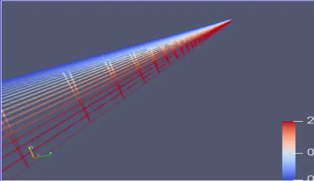
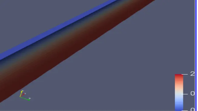
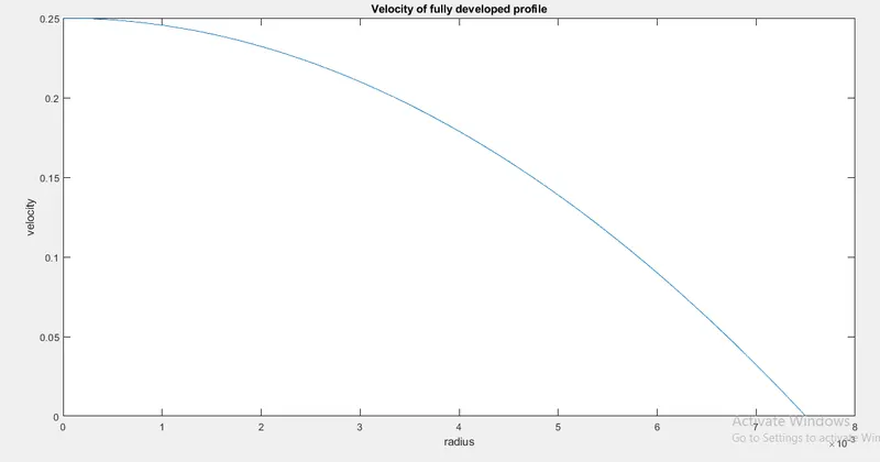
Analytical fully developed velocity profile :
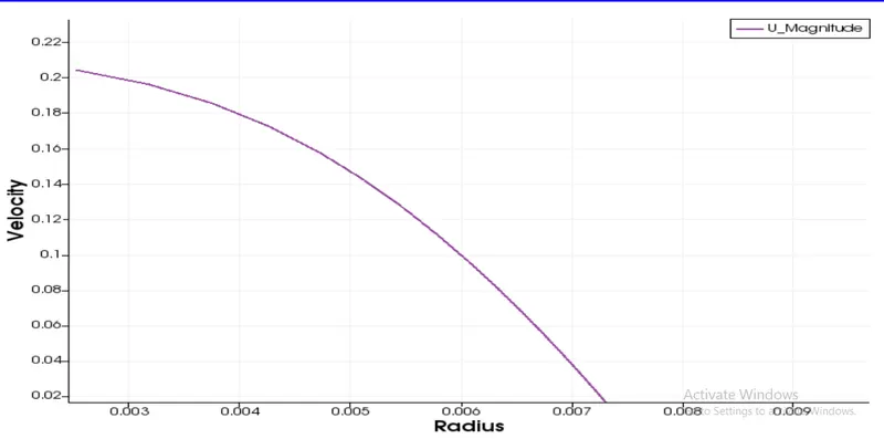
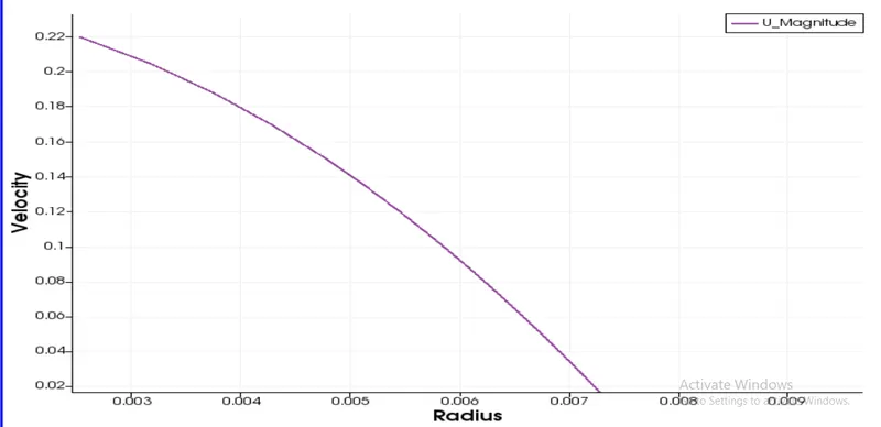
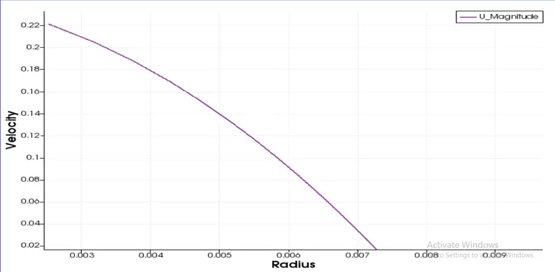
Velocity profiles at different lengths
at length 0.4 m
at length 1.575 m
at length 2.575 m
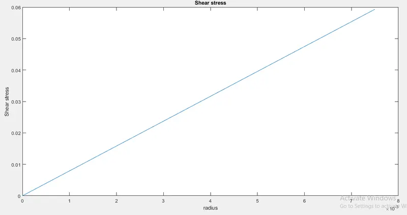
Now lets plot shear forces developed along the radius of the pipe
`tau = (2*mu*a*Vmax*)/(r^2)`
where
a is the particular point along the radius of the pipe
Shear stress plot
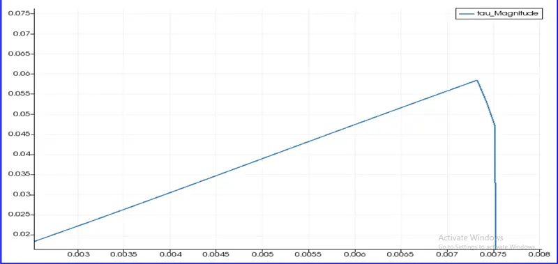
Now lets plot the shear stress vs radius from open foam and validate the results
Shear stress plot from openFoam
Results :
Calculated Maximum velocity : 0.25 m/sec
Maximum velocity from open foam : 0.22 m/sec
Maximum calculated shear stress : 0.006 Pascal
Maximum shear stress from openFoam : 0.007 Pascal