Week 7: Shock tube simulation project

Aim

To conduct a transient flow simulation on the given shock tube geometry to visualize the compression waves and analyze the temporal variations of pressure and temperature inside.

Introduction

The shock tube is an experimental facility that is used to replicate a blast wave or compression wave on a small scale. The shock tube is often used in research involving chemical kinetics and compressible flow phenomena. The working of a shock tube involves a high-pressure region and a low-pressure region separated by a diaphragm. When the diaphragm ruptures due to the increased pressure difference, the air from the high-pressure region gets sucked quickly into the low-pressure region creating shockwaves that propagate along the shock tube.

In the current study, a numerical simulation of the shock tube was conducted to visualize the compression waves and analyze the temporal variations of temperature and pressure inside the shock tube.

Method

Domain and Mesh

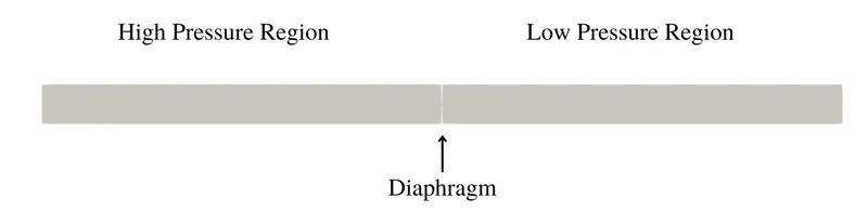
The geometry of the shock tube domain was provided and can be seen in the image below. The length of the shock tube was 0.2m with a width and height of 0.01m. The high-pressure and low-pressure region in the domain was separated by disconnected triangles which will be opened at time t=0.0001s which is the breaking of the diaphragm.

An unstructured cartesian grid was generated over the geometry with a sizing of 0.005m and the resulting base mesh contained 16k cells as seen below. Adaptive mesh refinement was conducted on the base mesh using a scaling factor of 3 and subgrid-scale criteria for N2 species set to 0.001.

CFD Setup

All Simulations were conducted using Converge v3.0. The fluid used in the domain was air with default properties. All walls in the domain were set to the slip boundary condition. The high-pressure region was initialized with a pressure of 6 bar, a temperature of 300K, and an N2 mass fraction of 1.0. The low-pressure region was initialized with a pressure of 1 bar, a temperature of 300K, and an N2 mass fraction of 0.

At time t=0s, the triangles between high-pressure and low-pressure regions were closed. At t=0.0001s, the triangles were set to deactivate and open the flow from the high-pressure to the low-pressure region.

The transient density-based PISO solver was used for the spatial discretization of the flow parameters. Turbulence in the flow was estimated using the two-equation RNG K-Epsilon Model. Momentum, density, turbulence, energy, and species were estimated using the SOR scheme while pressure was estimated using the converge bicgstab scheme.

The variable time stepping method was used for the simulation with minimum and maximum time step sizes of 1e-7s and 1s respectively. The max CFL number of the system was limited to 1. The simulation was conducted for a total time of 0.003s.

Results

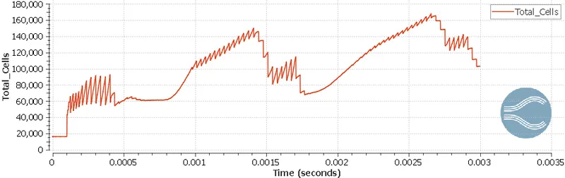
The image below shows the variations in the total cell count with time. The increase and decrease in the cell count are due to the adaptive mesh refinement identifying variations of N2 species in the domain.

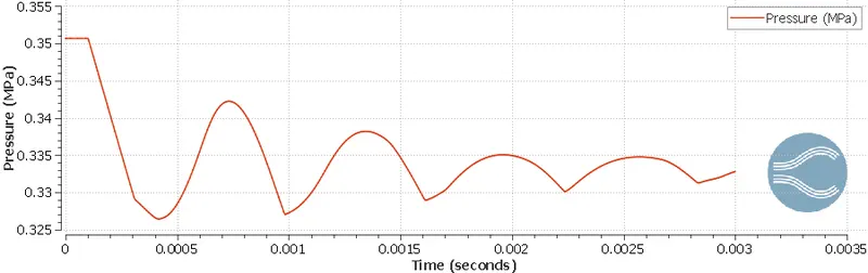
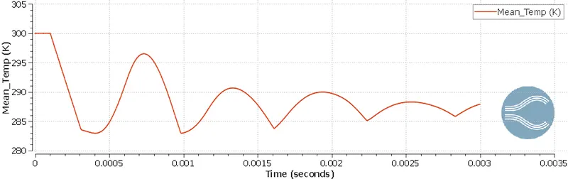
The images below show the variations in the average pressure and temperature of the domain with time. It can be seen that the amplitude of the pressure/temperature signals slowly decreases with time as they converge to a particular steady-state value. If the simulation is conducted for a longer time period, the steady-state pressure and temperature in the domain may be achieved.

Drive link to animations:

1. https://drive.google.com/file/d/1RJpwJhqaiIvO-nrmD-FS9OERwgaRZGUP/view?usp=sharing
   

   The first animation shows the variations of the mesh due to adaptive mesh refinement along with the distribution of N2 mass fraction in the domain. This animation provides a clear understanding of the working of the adaptive mesh refinement as it refines the regions of local fluctuations in N2 mass fractions.

   
   
   
2. https://drive.google.com/file/d/1tdZFRRVDVYMbDU2x2V9HbHI10ZNmgD9V/view?usp=sharing
   
   
   The second animation shows the variations in velocity and pressure in the domain. Compression waves can be seen to propagate from the high-pressure region to the lower-pressure region and are also seen to reflect from the walls of the domain. This animation clearly evidences the compression/pressure waves driving the velocity fields in the shock tube. It can also be seen that as the pressure in the domain decreases with time, the velocity in the domain also drops.
   

Conclusion

The transient flow simulation on the given shock tube geometry was conducted using converge. An adaptive mesh refinement was implemented based on variations of N2 species to capture the flow. Temporal variations of pressure and temperature in the domain were observed to converge to a steady state. Animations of variation of mesh, velocity, and pressure were used to visualize the compression waves flow in the shock tube.