Week 7: Shock tube simulation project
AIM: To simulate a transient shock tube using CONVERGE CFD.
OBJECTIVE:
- To plot the pressure and temperature history in the entire domain.
- To plot cell count as a function of time.
INTRODUCTION:
- Shock tubes are ideal devices for studying combustion and chemical kinetics at high temperature and pressure.
- These devices produce these conditions by generating a shock wave to compress and then heat the gas.
- A shock tube generates a shock wave using a section of high pressure gas and a section of low pressure gas separated by diaphragm.
- Once the diaphragm ruptures ,the driver and driven gases comes into contact ,creating a contact surface that act as a piston compressing the test gas and initiating shock wave propagation.
- The shock wave travels abd then reflects from the closed end wall of the shock tube causing further heating and compression of the test gas.
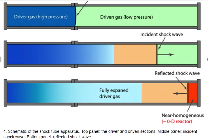
- Shock tubes are applied to the study of gas phase reactions on the milisecond time scale at temperature of several thousand kelvin.
- These are used for chemical kinetics measurements including ignition delay time,species time histories and determination of elementary reaction rates.
CASE SET UP
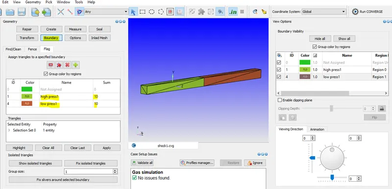
Fig.1 Boundary flagging
- In this set up we have taken hifh and low pressure as two boundary and are assigned to region 0 and 1 respectively.
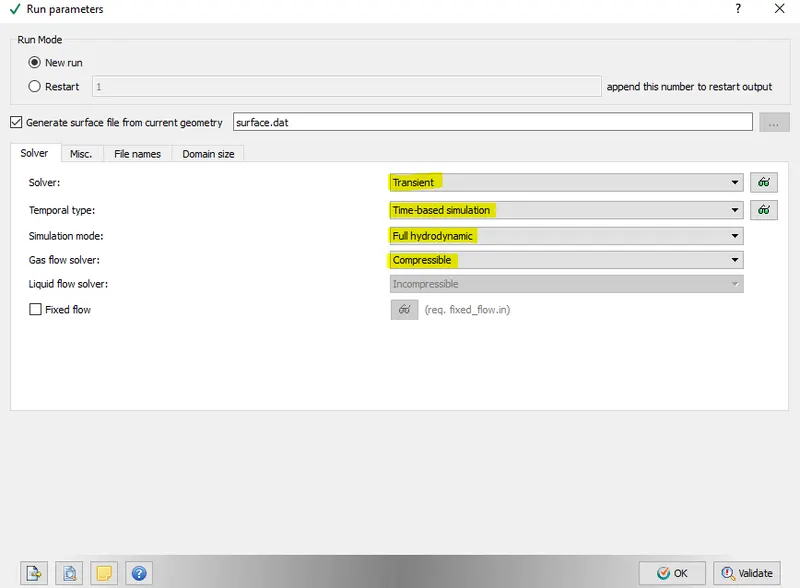
Fig.2 run parameter case set up
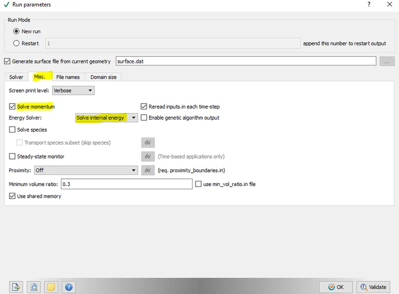
Fig.3 run parameter case set up
- Here uncheck the solve species and steady state monitor as we are simulating transient analysis.
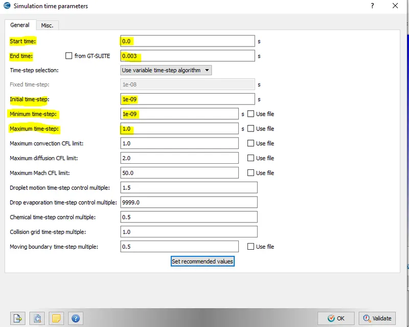
Fig.4 Simulation time parameter case set up.
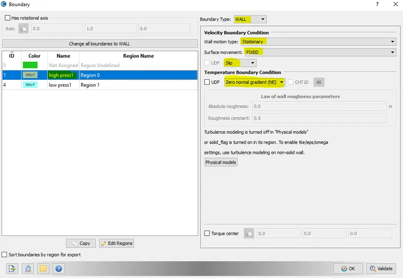
Fig.5 Boundary case set up
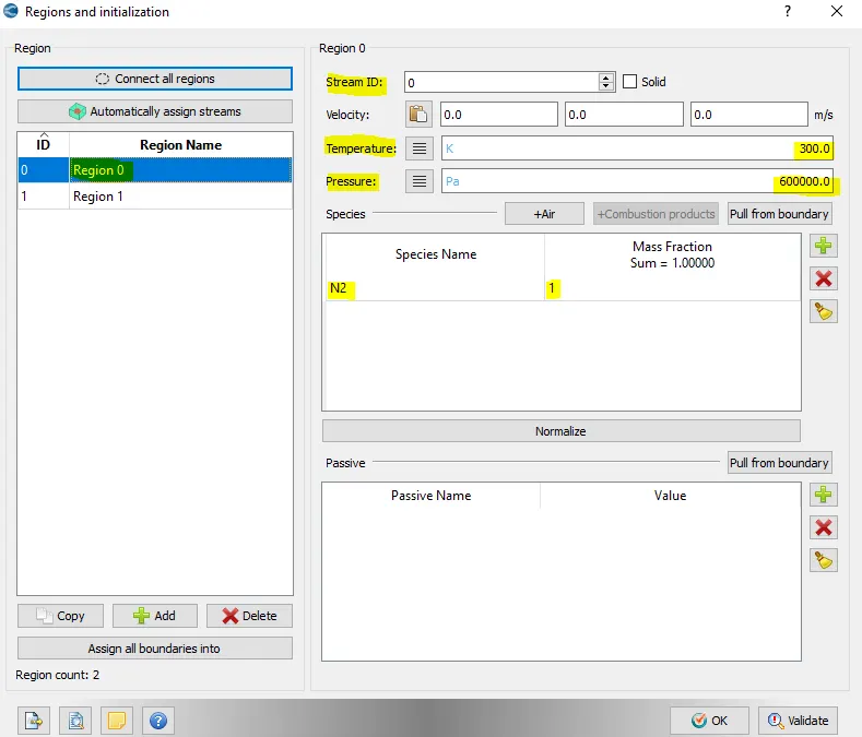
Fig.6 regions and initialization
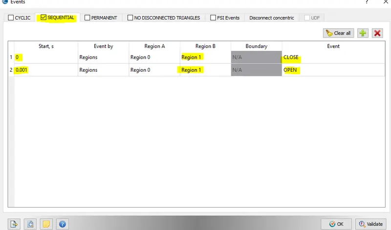
Fig.7 Events case set up
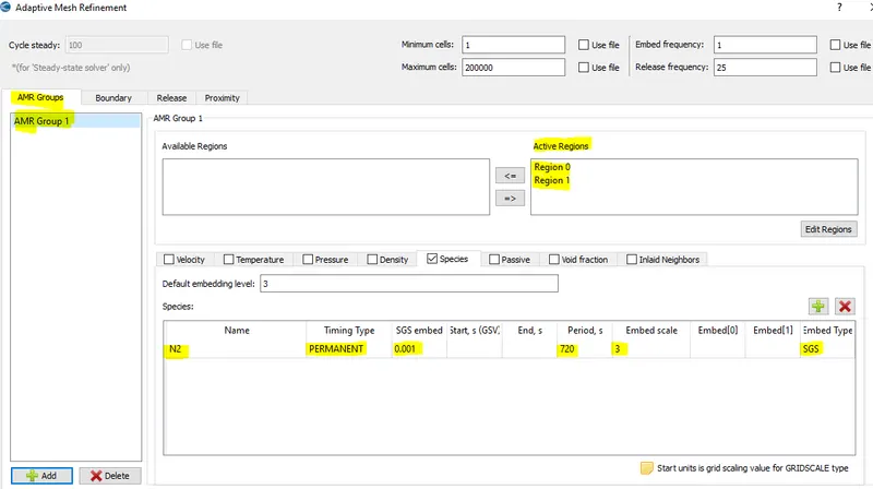
Fig.8 Adaptive mesh refinement
EVENTS
| START | REGION A | REGION B | EVENT |
| 0 | HIGH-PRESSURE | LOW-PRESSURE | CLOSE |
| 0.001 | HIGH-PRESSURE | LOW-PRESSURE | OPEN |
RESULTS
PLOTS
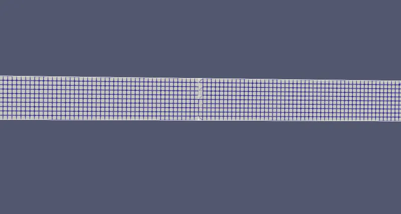
Fig.9 grid size (2mm mesh size)
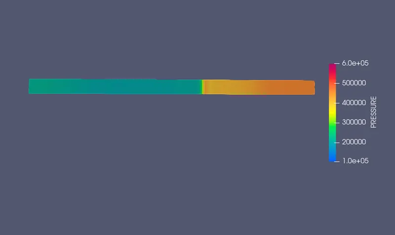
Fig.10 Pressure contour
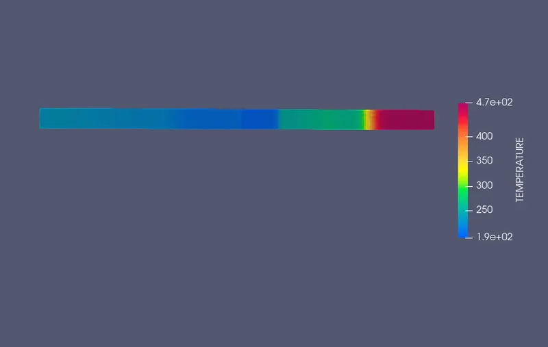
Fig.11 temperature contour
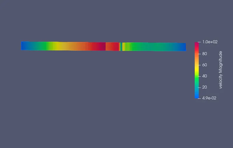
Fig.12 Velocity contour
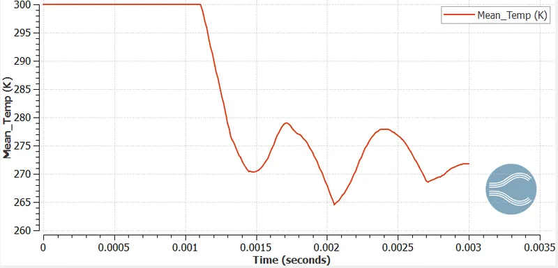
Fig.13 Mean temp.(k) vs time(sec)
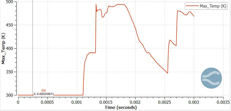
Fig.14 Max. temp.(k) vs time(sec)
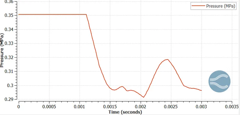
Fig.15 Pressure (MPa) vs time(sec)
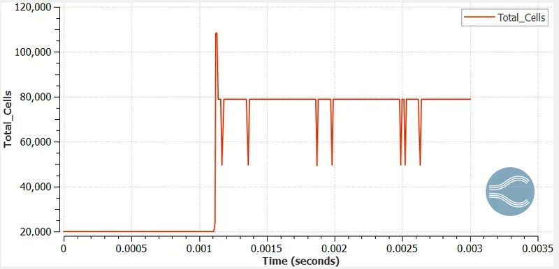
Fig.16 Total cell vs time(sec)
- As seen in the above plot ,when the event starts as open the total cell count drastically increases to a maximum level (hundred thousand).At this instance of time there is pressure gradient ,so the reaction taking place.
- Due to adaptive mesh refinement the cell count also increases as we have sub-grid species 0.001.
- Temperature animation
- velocity animation
- Pressure animation
CONCLUSION
- The transient simulation of shock tube is studied and results are post processed in paraview.
- The cell count increases as the event starts.
- The species mass fraction is captured using adaptive mesh refinement.
- The temperature and pressure plot shows at the beginning there is high pressure and temp. rise due to shock wave propagation and then as the wave gets reflected after seusequent time ,the value decreases.