Week 9 - FVM Literature Review

FINITE VOLUME METHOD:

• It is a method for representing and evaluating PDE in the form of algebraic equations.
• In finite volume method ,volume integrals in a PDE that contain a divergence term are converted to surface integrals using the divergence theorem.Divergence represents volume density of the outward flux of a vector field from an infinitesimal volume given at a point.

Divergence theorem:In vector calculus divergence theorem also known as Gauss' theorem which relates the flux of a vector field through a closed surface to the divergence of the field in the volume enclosed.

The volume rate of flow of liquid through a source or sink is equal to the divergence of the velocity field at the pipe mouth, so adding up the divergence of the liquid throughout the volume enclosed by 'S' equals the volume rate of flux through 'S'.

`intintint_V (grad.F)dV=ointoint_S (F.hatn)dS`

(volume integral over the volume V) (surface integral over the boundary of the volume V, represents total flow

(represents total of the sources in the volume V) across the boundary S)

• Divergence terms are then evaluated as fluxes at the surfaces of each finite volume.
• It is easily formulated for unstructured meshes.
• Finite volume refers to the small volume surrounding each node point on a mesh.

Basically when we have a practically problem of interest, first we need to identify the governing equation that govern the particular problem.So, physical problem either fluid flow or heat transfer problem then we should figure out set of governing equation.Once we get the set of governing equation(essentially PDEs),so these PDEs actually provide the solution for the that practical problem.These representative PDEs now needs to be converted to the linear system and then linear solvers are needed to solve them.

Generally finite difference method uses

• orthogonal grid
• discretization may not be necessarily conservative.

To overcome this problem,we use FVM to discretize the governing equation.In FVM the solution domain is sub-divided into a finite number of small non-overlapping control volume by a grid.This method inheriently conserve the basic conservation of governing variables.

• This method is extended to complex geometry where we have arbitrary control volume.
• In FVM ,we use normal which is outside the C.V,i.e,considered as positive.

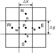
Fig.1

Now let us consider a two dimensional grid having cell named as N,S,W and E respectively. The grid spacing in X and Y direction as `DeltaX`and `DeltaY` respectively.

Now let us calculate the surface area vector of each face.

`S_e =A_e .i=DeltaY.i` , `S_w=-A_w.i=-DeltaY.i` , `S_n=A_n.j=DeltaX.j` , `S_s=-A_s.j=-DeltaX.j`

Need for Interpolation Scheme

The approximations of surface and volume integrals require values of the variables at locations other than the computational nodes of the control volume.Values at these locations are obtained by using interpolation formulae.

Various Interpolation Schemes

1. Upwind interpolation
2. Linear interpolation
3. Quadratic Upwind interpolation
4. Hybrid,TVD(Total Variable Diminishing) and ENO(Essentially Non Oscillatory Interpolation Scheme)

Upwind interpolation scheme:

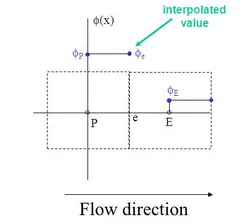
Fig.2

• Used for convection dominated problem.
• upwind interpolation scheme is equivalent to using a backward or forward finite difference approximation(depending on flow direction).

From the above figure ,the flow direction is shown by the arrow mark,so the function value at the eastern face:

`phi_e=phi_p` if `F_e>0`, `(vecV.vecn)_e >0`

= `phi_e` if `F_e<0` `(vecV.vecn)_e<0`

so using Taylor's series approximation

`f(x)=f_p+(x-x_p)((delf)/(delx))_p +(x-x_p)^2.((del^2f)/(delx^2))+......`

therefore value of function at eastern face:

`f_e=f_p+(x_e-x_p).((delf)/(delx))+(x_e-x_p)^2.((del^2f)/(delx^2))_p+.......`

• upwind scheme is first order approximate, introduces numerical diffusivity in our solution process.

`Gamma_d=rho.u(x_e-x_p)`

(numerical difusion co-efficient

• Upwind interpolation is the only approximation that satisfies boundedness criterion unconditionally, i.e(irrespective of velocity and grid spacing will never yield oscillatory solution).

some drawbacks....

• numerically diffusive :sharp peaks or oscillation which are actually present in the solution will be damped out.
• 1st order accurate : fine grids are required.

Linear interpolation scheme( central difference scheme):

• Approximate the value of the variable at control volume face center by linear interpolation of the values at two nearest computational nodes.
• It is 2nd order accurate.
• It may produce oscillatory solutions (advection dominated situation).
• Most widely choosen interpolation scheme specialy fine spatial and temporal grid spacing.
• Leads to a very simple approximation for evaluation of gradients required for evaluation of diffusive fluxes.
• pproximation of gradients has 2nd order accuracy on uniform grids.
• It's formally of first order on non-uniform grids.

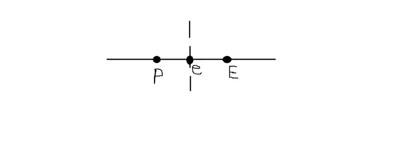
Fig.3

`f_e=f_E.lambda_e+f_p(1-lambda_e)` `lambda_e=(x_e-x_p)/(x_E-x_p)`

now `f_e=f_p+(x_e-x_p).((delf)/(delx))_p +(x_e-x_p)^2/2.((del^2f)/(delx^2))_p+.....` (1)

then functional value at node E in terms of Taylor's series around node P:

`f_E=f_p+(x_E-x_p)((delf)/(delx))_p+(x_E-x_p)^2/2.((del^2f)/(delx^2))_p+......` (2)

Quadratic Interpolation:

• Approximate the value of the variable at CV face centre by quadratic interpolation of the values at three nearest computationall nodes.
• It is third order accurate on both uniform and non-uniform grids.
• It is also named as QUICK(Quadratic Upwind Interpolation for convective kinematics)

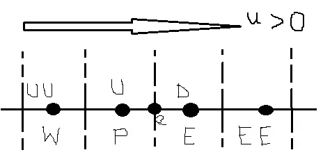
Fig.4

• From the above figure , let us consider nodes as W,P,E,EE.

UU=up upstream W= western cell

U= upstream E= eastern cell

D=downstream EE= eastern eastern cell

• we are considering the flow as the arrow mark is shown i.e from left to right along +ve x axis.

if `U_e>0` if `U_e<0`

then D=E, U=P, UU=W then D=P, U=E,UU=EE

• the functional value at node 'e'

`f_e=f_u+g_1.(f_D-f_U)+g_2.(f_(UU)-f_U)` where `g_1=((x_e-x_U).(x_e-x_(UU)))/((x_D-x_U).(x_D-x_(UU))`

`g_2=((x_e-x_U).(x_e-x_D))/((x_(UU)-x_U).(x_(UU)-x_D)`

• approximate function F by Quadratic Interpolation `F(x)=a_0+a_1.(x-x_u)+a_2.(x-x_u)` ..........(1)

at `x=x_u` , `F(u)=a_0` ................................(2)

similarly `F_D=a_0+a_1.(x_D-x_u)+a_2.(x_D-x_u)^2` then rearrange the term and write linear equation :

`a_1.(x_D-x_U)+a_2(x_D-x_U)^2=f_D-f_U` ...................................................................(3)

similarly at `x=x_(UU)`

`F_(UU)=F_(U)+a_1.(x_(UU)-x_U)+a_2.(x_(UU)-x_U)^2`

• now re-arrange the terms we get:

`a_1.(x_(UU)-x_U)+a_2(x_(UU)-x_U)^2=F_(UU)-F_U` ..............................................(4)

`[[F_D-F_U,(x_D-x_U)^2],[F_(UU)-F_U,(x_(UU)-x_U)^2]]`/(D) =`a_1`

where D= det `[[x_D-x_U,(x_D-x_U)^2],[x_(UU)-x_U,(x_(UU)-x_U)^2]]`

so,substituting the values of `a_1 and a_2` in interpolation we get :

`F_e=F_U+a_1.(x_e-x_U)+a_2.(x_e-x_U)^2`

now let us take an example of 1 dimensional linear heat conduction equation:

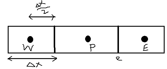
Fig.5

Integral form of governing equation:

`int_V(del/(delx)(alpha.(delT)/(delx))+S)dV=0`

`int_V(del/(delx)(alpha.(delT)/(delx))+bars)dV=0`

`int_V(del/(delx)(alpha.(delT)/(delx))dV+int_VsdV=0`

`int_(V=P) del/(delx)(alpha.(delT)/(delx))A.dx+int_VsdV=0`

`alpha_eA((T_e-T_p))/(Deltax)-alpha_w.A((T_p-T_w))/(Deltax)+barSdV=0`

(heat flux) (heat flux) (source term)

Need for Flux limiter

• The main role for flux limiter is to minimise the numerical dissipation.
• The idea of flux limiter is to address the source of oscillation.
• The source of oscillation is actually the extrapolation and any time we perform the extrapolation, we introduce potentially overshoots and undershoots.
• To minimise this we need scheme such as TVD(Total variation diminishing).It has to do to ensure that no new maximum cell average and no new minimum cell average value is present (which is analytical behaviour of scalar conservative laws).

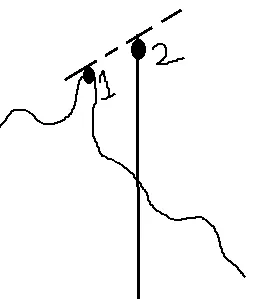
Fig.6

• Here in this fig.6, let us consider solution graph is having cell maximum value at point 1 and if we extrapolate the value of function at point 2 ,it might get a new local maximum value or overshoot the next cell average value.We should limit the gradient to something smaller value.

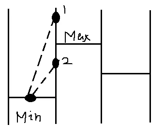
Fig.7

• In this figure it is clearly shown that there are 3 cell having their respective cell average values .let us consider for 1st cell ,it has minimum cell average value and if extrapolate the values near boundaries i.e, at point 1 or 2,if we are getting the value at point 2, then no need for reconstruction and if it is at point 1,then we have to modify it.
• flux limiter is a mechanism that detects local minimum and local maximum ,if cell average is higher than its left and right neighbour.