Week 3.5 - Deriving 4th order approximation of a 2nd order derivative using Taylor Table method

AIM:

To derive the following 4th order approximations of the second-order derivative.

1. Central difference

2. Skewed right-sided difference

3. Skewed left-sided difference

objective: To write a program in matlab to evaluate the second order derivative of the analytic function exp(x)*cos(x) and comparing it with three other approximation .

stencil for right skewed scheme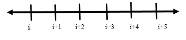

As shown in the figure, for right skewed scheme we have to take 6 grid points.The formula for finding the number of grid points is as follows:

N= number of nodes

P= order of accuracy

Q= order of derivative

N=P+Q, for 4th order approximation P=4 and Q=2 for 2nd order derivative

so N=4+2=6

TAYLOR TABLE

	f(i)	Δxf'(i)	Δx^2f''(i)	Δx^3f'''(i)	Δx^4f^(iv)(i)	Δx^5f^(v)(i)
af(i)	a	0	0	0	0	0
bf(i+1)	b	b	b/2	b/6	b/24	b/120
cf(i+2)	c	2c	4c/2	8c/6	16c/24	32c/120
df(i+3)	d	3d	9d/2	27d/6	81d/24	243d/120
ef(i+4)	e	4e	16e/2	64e/6	256e/24	1024e/120
gf(i+5)	g	5g	25g/2	125g/6	625g/24	3125g/120
summation	0	0	1	0	1	0

stencil for left skewed scheme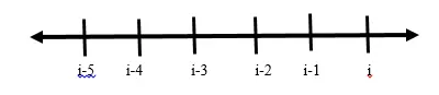

As shown in the figure, for Left skewed scheme we have to take 6 grid points.The formula for finding the number of grid points is as follows:

N= number of nodes

P= order of accuracy

Q= order of derivative

N=P+Q, for 4th order approximation P=4 and Q=2 for 2nd order derivative

so N=4+2=6

TAYLOR TABLE

	f(i)	Δxf'(i)	Δx^2f''(i)	Δx^3f'''(i)	Δx^4f^(iv)(i)	Δx^5f^(v)(i)
af(i)	a	0	0	0	0	0
bf(i-1)	b	-b	b/2	-b/6	b/24	-b/120
cf(i-2)	c	-2c	4c/2	-8c/6	16c/24	-32c/120
df(i-3)	d	-3d	9d/2	-27d/6	81d/24	-243d/120
ef(i-4)	e	-4e	16e/2	-64e/6	256e/24	-1024e/120
gf(i-5)	g	-5g	25g/2	-125g/6	625g/24	-3125g/120
summation	0	0	1	0	0	0

stencil for central difference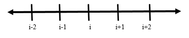

As shown in the figure, for Central difference scheme we have to take 5 grid points.The formula for finding the number of grid points is as follows:

N= number of nodes

P= order of accuracy

Q= order of derivative

N=P+Q-1, for 4th order approximation P=4 and Q=2 for 2nd order derivative

so N=4+2-1=5

TAYLOR TABLE

	f(i)	Δxf'(i)	Δx^2f''(i)	Δx^3f'''(i)	Δx^4f^(iv)(i)
af(i-2)	a	-2a	4a/2	-8a/6	16a/24
bf(i-1)	b	-b	b/2	-b/6	b/24
cf(i)	c	0	0	0	0
df(i+1)	d	d	d/2	d/6	d/24
ef(i+2)	e	2e	4e/2	8e/6	16e/24
summation	0	0	1	0	0

code for solving the system of equation using linsolve command in Matlab for calculating the coefficient matrix

% skewed_right_coefficient
clear all
close all
clc

A=[1 1 1 1 1 1;
    0 1 2 3 4 5;
    0 1/2 4/2 9/2 16/2 25/2;
    0 1/6 8/6 27/6 64/6 125/6;
    0 1/24 16/24 81/24 256/24 625/24;
    0 1/120 32/120 243/120 1024/120 3125/120;];
B=[0;0;1;0;0;0];
X=linsolve(A,B);


%central_difference_coefficient
C=[1 1 1 1 1;
    -2 -1 0 1 2;
    4/2 1/2 0 1/2 4/2;
    -8/6 -1/6 0 1/6 8/6;
    16/24 1/24 0 1/24 16/24;];
D=[0;0;1;0;0];
Y=linsolve(C,D);

% skewed_left_coefficient
E=[1 1 1 1 1 1;
    0 -1 -2 -3 -4 -5;
    0 1/2 4/2 9/2 16/2 25/2;
    0 -1/6 -8/6 -27/6 -64/6 -125/6;
    0 1/24 16/24 81/24 256/24 625/24;
    0 -1/120 -32/120 -243/120 -1024/120 -3125/120;];
F=[0;0;1;0;0;0];
Z=linsolve(E,F);

skewed right coefficient

skewed_right_coefficient


X =

    3.7500
  -12.8333
   17.8333
  -13.0000
    5.0833
   -0.8333

central difference coefficient

central_differene=coefficient

Y =

   -0.0833
    1.3333
   -2.5000
    1.3333
   -0.0833

skewed left coefficient

skewed_left_coefficint


Z =

    3.7500
  -12.8333
   17.8333
  -13.0000
    5.0833
   -0.8333

Main_program

main_program



clear all 
close all 
clc
% input variable
x=pi/3;
dx=linspace(pi/10,pi/3000,100);
for i=1:length(dx)
    skewed_left(i)=skewed_left_difference(x,dx(i));
    skewed_right(i)=skewed_right_difference(x,dx(i));
    central_diff(i)=central_difference(x,dx(i));
    FDS(i)=forward_difference(x,dx(i));
    BDS(i)=backward_difference(x,dx(i));
end
% plotting the figure
figure(1)
subplot(1,2,1)
loglog(dx,skewed_left,'r','linewidth',0.5,'marker','pentagram')
hold on
xlabel('dx')
ylabel('error')
loglog(dx,skewed_right,'b','linewidth',0.5,'marker','pentagram')
hold on
xlabel('dx')
ylabel('error')
loglog(dx,central_diff,'g','linewidth',0.5,'marker','pentagram')
legend('skewed_left','skewed_right','central_diff')
subplot(1,2,2)
loglog(dx,FDS,'r','linewidth',0.5,'marker','pentagram')
hold on
xlabel('dx')
ylabel('error')
loglog(dx,BDS,'b','linewidth',0.5,'marker','pentagram')
xlabel('dx')
ylabel('error')
legend('FDS','BDS')

function_code_for_skewed_right_scheme

function_code_for_skewed-right_scheme



% functiion_code
function skewed_right=skewed_right_difference(x,dx)
analytic_function=exp(x)*cos(x);
analytic_derivative=-2*exp(x)*sin(x);
%skewed_right_difference_coefficient
A=[1 1 1 1 1 1;
    0 1 2 3 4 5;
    0 1/2 4/2 9/2 16/2 25/2;
    0 1/6 8/6 27/6 64/6 125/6;
    0 1/24 16/24 81/24 256/24 625/24;
    0 1/120 32/120 243/120 1024/120 3125/120;];
B=[0;0;1;0;0;0];
X=linsolve(A,B);
skewed_right_difference=(X(1)*exp(x)*cos(x)+X(2)*exp(x+dx)*cos(x+dx)+X(3)*exp(x+(2*dx))*cos(x+(2*dx))+X(4)*exp(x+(3*dx))*cos(x+(3*dx))+X(5)*exp(x+(4*dx))*cos(x+(4*dx))+X(6)*exp(x+(5*dx))*cos(x+(5*dx)))/dx^2;
skewed_right=abs(skewed_right_difference-analytic_derivative);
end

function_code_for_skewed_left_scheme

function_code_forskewed_left-scheme


% functiion_code
function skewed_left=skewed_left_difference(x,dx)
analytic_function=exp(x)*cos(x);
analytic_derivative=-2*exp(x)*sin(x);
%skewed_right_difference_coefficient
E=[1 1 1 1 1 1;
    0 -1 -2 -3 -4 -5;
    0 1/2 4/2 9/2 16/2 25/2;
    0 -1/6 -8/6 -27/6 -64/6 -125/6;
    0 1/24 16/24 81/24 256/24 625/24;
    0 -1/120 -32/120 -243/120 -1024/120 -3125/120;];
F=[0;0;1;0;0;0];
Z=linsolve(E,F);
skewed_left_difference=(Z(1)*exp(x)*cos(x)+Z(2)*exp(x-dx)*cos(x-dx)+Z(3)*exp(x-2*dx)*cos(x-2*dx)+Z(4)*exp(x-3*dx)*cos(x-3*dx)+Z(5)*exp(x-4*dx)*cos(x-4*dx)+Z(6)*exp(x-5*dx)*cos(x-5*dx))/dx^2;
skewed_left=abs(skewed_left_difference-analytic_derivative);
end

function_code_for_central_difference

function_code_for_central_difference


%functional code
function central_diff=central_difference(x,dx)
analytic_function=exp(x)*cos(x);
analytic_derivtive=-2*exp(x)*sin(x);
%central_difference_coefficient
C=[1 1 1 1 1;
    -2 -1 0 1 2;
    4/2 1/2 0 1/2 4/2;
    -8/6 -1/6 0 1/6 8/6;
    16/24 1/24 0 1/24 16/24;];
D=[0;0;1;0;0];
Y=linsolve(C,D);
central_difference=(Y(1)*exp(x-2*dx)*cos(x-2*dx)+Y(2)*exp(x-dx)*cos(x-dx)+Y(3)*exp(x)*cos(x)+Y(4)*exp(x+dx)*cos(x+dx)+Y(5)*exp(x+2*dx)*cos(x+2*dx))/dx^2;
central_diff=abs(central_difference-analytic_derivtive);
end

function_code_for_forward_differencing

function_code_for_forward_difference


function FDS=forward_difference(x,dx)
analytic_function=exp(x)*cos(x);
analytic_derivative=-2*exp(x)*sin(x);
forward_difference=(exp(x+dx)*cos(x+dx)-exp(x)*cos(x))/dx;
FDS=abs(forward_difference-analytic_derivative);

function_code_for_backward_differencing

function_code_for_backward_difference


function BDS=backward_difference(x,dx)
analytic_function=exp(x)*cos(x);
analytic_derivative=-2*exp(x)*sin(x);
backward_difference=(exp(x)*cos(x)-exp(x-dx)*cos(x-dx))/dx;
BDS=abs(backward_difference-analytic_derivative);

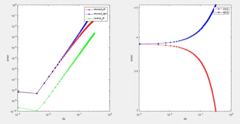
PLOT ON LOGLOG GRAPH

conclusion

• From the above plot ,it is shown that skewed right scheme is having more error as compared to skewed left and central difference scheme.
• As the grid spacing decreases, the error value for skewe right and skewed left shown in plot remains almost same.CDS is having lower error values than other two schemes.
• Here the CDS,skewed right and skewed left are 2nd order derivative and 4th order approximation, accuracy point of view if we see then CDS is more accurate as it is taking both left and right side grid points into consideration.
• In FDS and BDS the error value is going to a minimum when we will take finer grid points.

why a skewed scheme is useful? What can a skewed scheme do that a CD scheme cannot?

skewed scheme is useful for evaluating the numerical approximation to differential equations.If we consider for an example the flow of fluids in pipe and in the entrance region say at x=0, if we want to take the grid points before the entrance region ,we end up with no information available for calculation.Because the domain we want for consideration is the entrance region(leading edge) to trailing edge. So for simulating the fluid flow ,we have to take the grid points x=0 to right side. Generally skewed scheme is useful when there is no information available on both side of the node .Whereas if we consider CDS, it is taking the information available at grid points from left and right of the nodes taken into consideration.