Week 7 - Simulation of a 1D Super-sonic nozzle flow simulation using Macormack Method

AIM:Simulation of 1-D super sonic nozzle flow using Maccormack method

OBJECTIVE

Need to show the following plots inside the report
1. Steady-state distribution of primitive variables inside the nozzle.
2. Time-wise variation of the primitive variables.
3. Variation of Mass flow rate distribution inside the nozzle at different time steps during the time-marching process.
4. Comparison of Normalized mass flow rate distributions of both forms.

Expected Results:

• Perform a grid independence test on the solution and expain all your findings.
• The code must be modular. You need to write separate functions to solve both forms.
• Discuss all the plots you are providing with observed inferences.

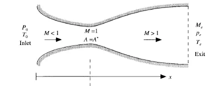
• In this problem ,we consider the steady ,isentropic flow through a convergent -divergent nozzle as sketched in above figure.
• The pressure and temperature at the inlet of the nozzle are denoted by `P_0`and `T_0` respectively.
• As the cross-sectional area of reservoir is large ,the velocity is very small (v`rarr`0).
• The flow expands isentropically to supersonic speeds at the nozzle exit.
• `P_e,T_e,V_e and M_e` are exit pressure,temperature,velocity and mach number respectively.
• The flow is sub-sonic in the convergent section,sonic at the throat and supersonic at the divergent section.
• Sonic flow is defined as the case when local velocity at a location is equal to local speed of sound.

ASSUMPTION

• Flow properties vary only with length of nozzle and assuming uniform flow properties across any given cross section ,such flow is quasi -one-dimensional flow.

Governing continuity,momentum and energy equation for this quasi-one dimensional ,steady,isentropic flow can be expressed as :

continuity equation:`rho_1V_1A_1=rho_2V_2A_2`

Momentum equation: `P_1A_1+rho_1V_1^2A_1+int_(A_1)^(A_2) PdA=P_2A_2+rho_2V_2^2A_2`

Energy equation: `h_1+V_1^2/2 =h_2+V_2^2/2`

Mach number variation through the nozzle is governed by area ratio: `(A/A^star)^2=(1/M^2)*(2/(gamma+1)*(1+(gamma-1)/2*M^2))^((gamma+1)/(gamma-1))`

• The force exerted on the gas to accelerate it through the nozzle is supplied by the pressure ratio across the nozzle `P_0/P_e`.For a nozzle with a specified area ratio `(A_e/A^star)`,the pressure ratio required to establish the subsonic-supersonic isentropic flow must be a specified value. the pressure ratio is provided by the high pressure air reservoir.

Writing the governing continuity,momentum and energy equation in non-dimensional term which is as follows:

Continuity equation: `(drho^')/dt^'=-rho^'*(dV^')/dx^' -rho^'*V^'*(dlnA^')/dx^' -V^'*(drho^')/dx^'`

Momentum equation: `(dV^')/dt^' =-V*(dV^')/dx^'-(1/gamma)*((dT^')/dx^'+(T^'/rho^')*(drho^')/dx^')`

Energy equation: `(dT^')/dt^' =-V^'*(dT^')/dx^' -(gamma-1)*T^'*((dV^')/dx^'+V^'*(dlnA^')/dx^')`

• As we know, the reservoir temperature and density are denoted by `T_0` and `rho_0` respectively,we define the non-dimensional temperature and density respectively as `T^'=T/T_0` and `rho^'=rho/rho_0`

Here the prime denotes a dimensionless variable.

similarly the dimensionless length `x^'=x/L` where L=length of the nozzle .

• As `a_0` the speed of sound in the reservoir then `a_0=sqrt(gamma*R*T_0)` then dimensionless velocity as

`V^'=V/a_0`.

Then the quantity (`L/a_0`) has dimension of time, so dimensionless time `t^'=(t/(L/a_0))` and

dimensionless area `A^'=A/A^star`

• MACCORMACK TECHNIQUE

1. predictor step
2. corrector step

• It is an explicit finite-difference technique which is second order accurate in both space and time.
• In Maccormack technique the flow field variables are calculated as :

1. `rho_(i,j)^(t+Deltat) =rho_(i,j)^t +((delrho)/(delt))_(av) *Deltat` density at time step `t+Deltat`
   
2. `u_(i,j)^(t+Deltat) =u_(i,j)^t +((delu)/(delt))_(av)*Deltat` x-component of velocity at time step `t+Deltat`
3. `V_(i,j)^(t+Deltat)=V_(i,j)^t +((delV)/(delt))_(av)*Deltat` y-component of velocity at time step `t+Deltat`
4. `e_(i,j)^(t+Deltat) =e_(i,j)^(t) +((dele)/(delt))_(av)*Deltat` energy at time step `t+Deltat`

PREDICTOR STEP

• In this step we have to replace the spatial derivatives on the R.H.S with forward differences and we know all flow variables at time step 't' are known.

so, the predicted value of density is calculated from Taylor's series i.e(first two terms) :

`((drho)/(dt))_(i,j)^t=-((rho_(i,j)^t*(U_(i+1,j)^t-U_(i,j)^t)/(Deltax))+U_(i,j)*((rho_(i+1,j)^t-rho_(i,j)^t)/(Deltax))+(rho_(i,j)^t*(V_(i,j+1)^t-V_(i,j)^t)/(Deltay))+V_(i,j)^t*((rho_(i,j+1)-rho_(i,j)^t)/(Deltay)))` .......................(1)

• In a similar fashion the time derivatives on the R.H.S are obtained with forward differences for spatial derivatives.

so, `(u)_(i,j)^(t+Deltat)=U_(i,j)^t+((delu)/(delt))_(i,j)^t*Deltat`

`V_(i,j)^(t+Deltat)=V_(i,j)^t+((delV)/(delt))_(i,j)^t*Deltat`

CORRECTOR STEP

• In this step ,we have to substitute the predicted values of density ,velocity into the R.H.S of the continuity,momentum and energy equation at time step `t+Deltat`by replacing the spatial derivatives with rearward differences.

`((delrho)/(delt))_(i,jc)^(t+Deltat)=-(rho_(i,jp)^(t+Deltat)*(u_(i,j)^(t+Deltat)-u_(i-1,j)^(t+Deltat))/(Deltax)+u_(i,j)^(t+Deltat)*(rho_(i,j)^(t+Deltat)-rho_(i-1,j)^(t+Deltat))/(Deltax)+rho_(i,j)^(t+Deltat)*(V_(i,j)^(t+Deltat)-V_(i,j-1)^(t+Deltat))/(Deltay)+V_(i,j)^(t+Deltat)*(rho_(i,j)^(t+Deltat)-rho_(i,j-1)^(t+Deltat))/(Deltay))` ....................................(2)

• Then the average value of the time derivative of density is obtained from the arithematic mean of `((delrho)/(delt))_(i,j)^t` obtained from equation (1) and (2) as :

`((delrho)/(delt))_(av)=1/2*(((delrho)/(delt))_(i,j)^t+((delrho)/(delt))_(i,j)^(t+Deltat))` ........................................(3)

This procedure is repeated for all grid points to calculate the density at time step `(t+Deltat)` respectively.Similarly all other flow variables will be calculated as done in above equation.

NON CONSERVATION EQUATION

1. `((delrho^')/(dt^'))=-rho^'*(delV^')/(delx^')-rho^'*V^'*(dellnA^')/(delx^')-V^'*(delrho^')/(delx^')` ...........pressure
   
2. `(delV^')/(delt^')=-V^'*(delV^')/(delx^')-(1/gamma)*((delT^')/(delx^')+T^'/rho^'*(delrho^')/(delx^'))`.........velocity
3. `(delT^')/(delt^')=-V^'*(delT^')/(delx^')-(gamma-1)*T^'*((delV^')/(delx')+V^'*(dellnA^')/(delx^'))` ...........temperature

The non conservation equation is same as the continuity,momentum and energy equation in non-dimensional form.For predicted values we have to discretize the above equation for space terms in forward differencing approach and for corrector values we have to discretize the space terms in backward differencing.

CONSERVATIVE EQUATION

Governing equation are expressed in generic form which consists of the solution vector U,the flux vector F and the source term J

so, `(delU)/(delt) +(delF)/(delx)=J`

lets define the term `U_1=rho^'*A^'`

`U_2=rho^'*A^'*V^'`

`U_3=rho^'*A^'*(e^'/(gamma-1)+(gamma/2)*(V^')^2)`

`F_1=rho^'*V^'*A^'`

`F_2=rho^'*A^'*(V^')^2 +(1/gamma)*P^'*A^'`

`F_3=rho^'*V^'*A^'*(e^'/(gamma-1)+(gamma/2)*(V^')^2)`

`J_2=1/gamma*P^'*(delA^')/(delx^')`

and

`(delU_1)/(delt^')=-(delF_1)/(delx^')`

`(delU_2)/(delt^')=-(delF_2)/(delx^')+J_2`

`(delU_3)/(delt^')=-(delF_3)/(delx^')`

• for calculating the primitive variables (`rho,T,V,P`),we must decode the elements `U_1,U_2 and U_3` as shown

`rho^'=U_1/A^'` ,`V^'=U_2/U_1` , `T^'=e^'=(gamma-1)*((U_3/U_2)-gamma/2*(V^')^2)`

MAIN PROGRAM

clear all
close all
clc
% no. of grid points
n=31;
x=linspace(0,3,n);
% grid spacing
dx=x(2)-x(1);
% specific heat ratio
gamma=1.4;
% area
a=1+2.2*(x-1.5).^2;
% courant number
c=0.5;
nt=1400;
% analytical solution
rho_an=0.634*ones(900,1400);
T_an=0.833*ones(900,1400);
p_an=0.528*ones(900,1400);
M_an=1*ones(900,1400);
% function calling
% conservative
tic
[rho_con,T_con,v,dt,mac_con,p_con,mfr_con,rho_th,T_th,p_th,mac_th,mfr_th]=conservative(x,dx,n,gamma,c,nt,a);
conservative_time=toc;

tic
[rho,T,V,p,mfr_noncon,rho_throat,T_throat,p_throat,mac,mac_t,mfr_throat]=nonconservative(x,dx,n,c,gamma,nt,a);
nonconservative_time=toc;

figure(2)

subplot(6,1,1)
plot(x,v,'color','b','linewidth',2)
hold on
xlabel('length of nozzle')
ylabel('velocity ratio')
legend(' velocity ratio conservative')

subplot(6,1,2)
plot(x,T_con,'color','g','linewidth',2)
hold on
xlabel('length of nozzle')
ylabel('temperature ratio')
legend(' temperature ratio conservative')

subplot(6,1,3)
plot(x,rho_con,'color','y','linewidth',2)
hold on
xlabel('length of nozzle')
ylabel('density ratio')
legend(' density ratio conservative')

subplot(6,1,4)
plot(x,p_con,'color','r','linewidth',2)
hold on
xlabel('length of nozzle')
ylabel('press ratio')
legend('pressure ratio conservative')

subplot(6,1,5)
plot(x,mfr_con,'color','bla','linewidth',2)
hold on
xlabel('length of nozzle')
ylabel('mass flow rate')
legend('mass flow rate conservative')

subplot(6,1,6)
plot(x,mac_con,'color','m','linewidth',2)
hold on
xlabel('length of nozzle')
ylabel('mach number')
legend('mach number conservative')


figure(3)

subplot(6,1,1)
plot(x,p,'color','r','linewidth',1.5)
hold on
xlabel('non dimensional distance')
ylabel('pressure')
legend('pressure for nonconservative')
grid on

subplot(6,1,2)
plot(x,mac,'color','b','linewidth',1.5)
hold on
xlabel('non dimensional distance')
ylabel('mach number')
legend('mach number for nonconservative')
grid on

subplot(6,1,3)
plot(x,mfr_noncon,'color','g','linewidth',1.5)
hold on
xlabel('non dimensional distance')
ylabel('mass flow rate')
axis([0 3 0.5856 0.5990])
legend('mass flow rate for nonconservative')
grid on

subplot(6,1,4)
plot(x,V,'color','y','linewidth',1.5)
hold on
xlabel('non dimensional distance')
ylabel('velocity')
legend('velocity for nonconservative')
grid on

subplot(6,1,5)
plot(x,T,'color','bla','linewidth',1.5)
hold on
xlabel('non dimensional distance')
ylabel('temperature')
legend('temperature for nonconservative')
grid on

subplot(6,1,6)
plot(x,rho,'color','m','linewidth',1.5)
hold on
xlabel('non dimensional distance')
ylabel('density')
legend('density for nonconservative')
grid on


figure(4)

subplot(5,1,1)
plot(rho_th,'r')
hold on
plot(rho_throat,'b')
hold on
plot(rho_an,'g')
xlabel('time step')
ylabel('density')
legend('conservative','non-conservative','analytic')
title('variatio of flow properties with time step')

subplot(5,1,2)
plot(T_th,'r')
hold on
plot(T_throat,'b')
hold on
plot(T_an,'g')
xlabel('time step')
ylabel('temperature')
legend('conservative','non-conservative','analytic')
title('variatio of flow properties with time step')

subplot(5,1,3)
plot(p_th,'r')
hold on
plot(p_throat,'b')
hold on
plot(p_an,'g')
xlabel('time step')
ylabel('pressure')
legend('conservative','non-conservative','analytic')
title('variation of flow properties with time step')

subplot(5,1,4)
plot(mac_th,'r')
hold on
plot(mac_t,'b')
hold on
plot(M_an,'g')
xlabel('time step')
ylabel('mach number')
legend('conservative','non-conservative','analytic')
title('variation of flow properties with time step')

subplot(5,1,5)
plot(mfr_th,'r')
hold on
plot(mfr_throat,'b')
hold on
xlabel('time step')
ylabel('mass flow rate')
legend('conservative','non-conservative')
title('variation of flow properties with time step')


figure(6)
plot(x,mfr_con,'color','r','linewidth',1.5)
hold on
plot(x,mfr_noncon,'color','b','linewidth',1.5)
xlabel('non dimensional distance')
ylabel('mass flow rate')
legend('conservative','nonconservative')
title('variation of mass flow rate with non dim. distance')

FUNCTION CODE FOR CONSERVATIVE PART

unction [rho_con,T_con,v,dt,mac_con ,p_con,mfr_con,rho_th,T_th,p_th,mac_th]=conservative(x,dx,n,gamma,c,nt,a)

    for i=1:length(x)
    if x(i)>=0 && x(i)<=0.5
        rho_con(i)=1;
        T_con(i)=1;
    elseif x(i)>=0.5 && x(i)<=1.5
        rho_con(i)=1-0.366*(x(i)-0.5);
        T_con(i)=1-0.167*(x(i)-0.5);
    elseif x(i)>=1.5 && x(i)<=3
        rho_con(i)=0.634-0.3879*(x(i)-1.5);
        T_con(i)=0.833-0.3507*(x(i)-1.5);
    end
    end
%velocity
v=(0.59)./(rho_con.*a);
%pressure
p_con=(rho_con).*T_con;

U1=rho_con.*a;
U2=rho_con.*a.*v;
U3=rho_con.*a.*(T_con./(gamma-1)+(gamma/2).*v.^2);
dt=min(c.*dx./(sqrt(T_con)+v));
 %time loop
for k=1:nt
    U1_old=U1;
    U2_old=U2;
    U3_old=U3;
    
    F1=U2;
    F2=((U2.^2)./U1)+((gamma-1)/(gamma)*(U3-(gamma*U2.^2)./(2*U1)));
    F3=((gamma*U2.*U3)./U1)-((gamma*(gamma-1)/2)*((U2.^3)./U1.^2));
    % predictor method
    for j=2:n-1
        % continuity equation
         dU1dt_p(j)=-(F1(j+1)-F1(j))/dx;
         % momentum equation
        J2(j)=(1/gamma)*rho_con(j)*T_con(j)*((a(j+1)-a(j))/dx);
        dU2dt_p(j)=-(F2(j+1)-F2(j))/dx+J2(j);
        % energy equation
        dU3dt_p(j)=-(F3(j+1)-F3(j))/dx;
        % solution update
        U1(j)=U1(j)+dU1dt_p(j)*dt;
        U2(j)=U2(j)+dU2dt_p(j)*dt;
        U3(j)=U3(j)+dU3dt_p(j)*dt;
    end
    % updating the flux term 
    v=U2./U1;
    rho_con=U1./a;
    T_con=(gamma-1)*(U3./U1-(gamma/2)*v.^2);
    p_con=(rho_con).*T_con;
    
    
    F1=U2;
    F2=((U2.^2)./U1)+((gamma-1)/(gamma)*(U3-(gamma*U2.^2)./(2*U1)));
    F3=((gamma*U2.*U3)./U1)-((gamma*(gamma-1)/2)*((U2.^3)./U1.^2));
    % corrector method
    for j=2:n-1
        J2(j)=(1/gamma)*rho_con(j)*T_con(j)*((a(j)-a(j-1))/dx);
        %continuity equation
        dU1dt_c(j)=-(F1(j)-F1(j-1))/dx;
        %momentum equation
        dU2dt_c(j)=-(F2(j)-F2(j-1))/dx+J2(j);
        %energy equation
        dU3dt_c(j)=-(F3(j)-F3(j-1))/dx;
        
    end
    % compute the average time derivative
    dU1dt_avg=0.5*(dU1dt_p+dU1dt_c);
    dU2dt_avg=0.5*(dU2dt_p+dU2dt_c);
    dU3dt_avg=0.5*(dU3dt_p+dU3dt_c);
    % update the final solution
    for m=2:n-1
        U1(m)=U1_old(m)+dU1dt_avg(m)*dt;
        U2(m)=U2_old(m)+dU2dt_avg(m)*dt;
        U3(m)=U3_old(m)+dU3dt_avg(m)*dt;
    end
    
    U1(1)=rho_con(1).*a(1);
    U2(1)=(2*U2(2))-U2(3);
    U3(1)=U1(1)*(T_con(1)/(gamma-1)+(gamma/2)*v(1).^2);
    
    % apply the boundary condition
    U1(n)=2*U1(n-1)-U1(n-2);
    U2(n)=2*U2(n-1)-U2(n-2);
    U3(n)=2*U3(n-1)-U3(n-2);
    
    rho_con=U1./a;
    v=U2./U1;
    T_con=(gamma-1)*(U3./U1-(gamma/2)*v.^2);
    p_con=(rho_con).*T_con;
    mfr_con=rho_con.*v.*a;
    mac_con=v./(T_con).^0.5;
     
    figure(5)
    if k==50
        figure(5)
        plot(x,mfr_con,'b','linewidth',2)
        hold on
    elseif k==100
        figure(5)
        plot(x,mfr_con,'g','linewidth',2)
        hold on
    elseif k==300
        figure(5)
        plot(x,mfr_con,'r','linewidth',2)
        hold on
    elseif k==400
        figure(5)
        plot(x,mfr_con,'y','linewidth',2)
        hold on
        
    elseif k==700
        figure(5)
        plot(x,mfr_con,'bla','linewidth',2)
        hold on
    elseif k==1000
        figure(5)
        plot(x,mfr_con,'m','linewidth',2)
        hold on
        grid on
        legend('50time step','100time step','300time step','400time step','700time step','1000time step')
        xlabel('length of nozzle')
        ylabel('mass flow rate')
        axis([0 3 0 1])
        title('mass flow rate vs different time step for conservative method')
    end



    
    rho_th(k)=rho_con(16);
    T_th(k)=T_con(16);
    p_th(k)=p_con(16);
    mac_th(k)=mac_con(16);
end

FUNCTION CODE FOR NONCONSERVATIVE PART

function [rho,T,V,p,mfr_noncon,rho_throat,T_throat,p_throat,mac,mac_t]=nonconservative(x,dx,n,c,gamma,nt,a)

%calcuate initial profiles
rho=1-0.3146.*x;
% temperature
T=1-0.2314.*x;
% velocity
V=(0.1+1.09*x).*T.^0.5;
dt=min(c.*dx./(sqrt(T)+V));

    for k=1:nt
    %predictor method
    rho_old=rho;
    V_old=V;
    T_old=T;
    %continuity equation(for inner node)
    for j=2:n-1
%         drho_dt_p=-rho(j)*((V(j+1)-V(j))/dx)-rho(j)*V(j)*((log(A(j+1))-log(A(j)))/dx)-V(j)*(rho(j+1)-rho(j))/dx;
        dvdx=(V(j+1)-V(j))/dx;
        drhodx=(rho(j+1)-rho(j))/dx;
        dTdx=(T(j+1)-T(j))/dx;
        dlogadx=(log(a(j+1))-log(a(j)))/(dx);%continuity equation
        drhodt_p(j)=-rho(j)*dvdx-rho(j)*V(j)*dlogadx-V(j)*drhodx;
        %momentum equation
        dvdt_p(j)=-V(j)*dvdx-(1/gamma)*(dTdx+(T(j)/rho(j))*drhodx);
        %energy equation
        dTdt_p(j)=-V(j)*dTdx-(gamma-1)*T(j)*(dvdx+V(j)*dlogadx);
        %solution update
        rho(j)=rho(j)+drhodt_p(j)*dt;
        V(j)=V(j)+dvdt_p(j)*dt;
        T(j)=T(j)+dTdt_p(j)*dt;
    end

%corrector method
for j=2:n-1
    dvdx=(V(j)-V(j-1))/dx;
        drhodx=(rho(j)-rho(j-1))/dx;
        dTdx=(T(j)-T(j-1))/dx;
        dlogadx=(log(a(j))-log(a(j-1)))/(dx);%continuity equation
        drhodt_c(j)=-rho(j)*dvdx-rho(j)*V(j)*dlogadx-V(j)*drhodx;
         %momentum equation
        dvdt_c(j)=-V(j)*dvdx-(1/gamma)*(dTdx+(T(j)/rho(j))*drhodx);
        %energy equation
        dTdt_c(j)=-V(j)*dTdx-(gamma-1)*T(j)*(dvdx+V(j)*dlogadx);
end
% compute the average time derivative
drhodt=0.5*(drhodt_p+drhodt_c);
dvdt=0.5*(dvdt_p+dvdt_c);
dTdt=0.5*(dTdt_p+dTdt_c);
%final solution update

for m=2:n-1
rho(m)=rho_old(m)+drhodt(m)*dt;
V(m)=V_old(m)+dvdt(m)*dt;
T(m)=T_old(m)+dTdt(m)*dt;
end
% apply the boundary condition

V(1)=2*V(2)-V(3);
rho(1)=1;
T(1)=1;

V(n)=2*V(n-1)-V(n-2);
rho(n)=2*rho(n-1)-rho(n-2);
T(n)=2*T(n-1)-T(n-2);
% pressure
p=rho.*T;
%mass flow rate
mfr_noncon=rho.*a.*V;
%mach number
mac=V./(T).^0.5;
figure(1)
    if k==50
        figure(1)
        plot(x,mfr_noncon,'color','g','linewidth',2)
        hold on
    elseif k==100
        figure(1)
        plot(x,mfr_noncon,'color','b','linewidth',2)
        hold on
    elseif k==300
        figure(1)
        plot(x,mfr_noncon,'color','r','linewidth',2)
        hold on
    elseif k==400
        figure(1)
        plot(x,mfr_noncon,'color','bla','linewidth',2)
        hold on
    elseif k==700
        figure(1)
        plot(x,mfr_noncon,'color','y','linewidth',2)
        legend('50time step','100time step','300time step','400time step','700time step')
        xlabel('length of nozzle')
        ylabel('mass flow rate')
        axis([0 3 0 2])
        title('mass flow rate vs different time step for nonconservative method')
    end
    rho_throat(k)=rho(16);
    T_throat(k)=T(16);
    p_throat(k)=p(16);
    mac_t(k)=mac(16);
        
        
    end

Results

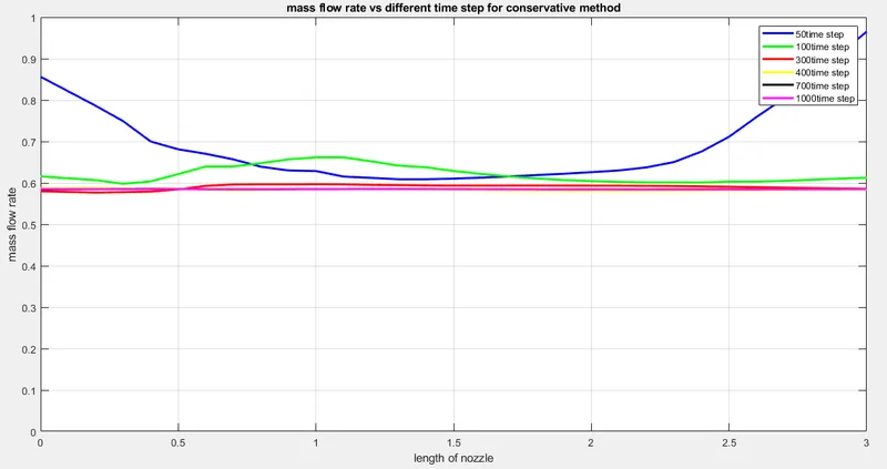
n=31

mass flow rate for different time step for conservative method

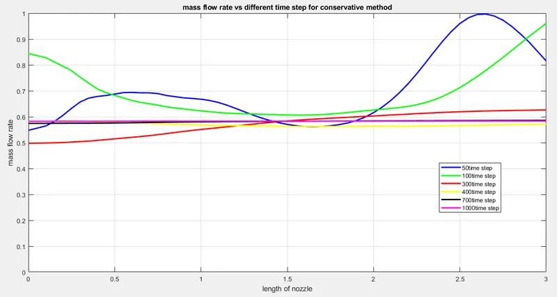
n=61

mass flow rate for different time step for conservative method

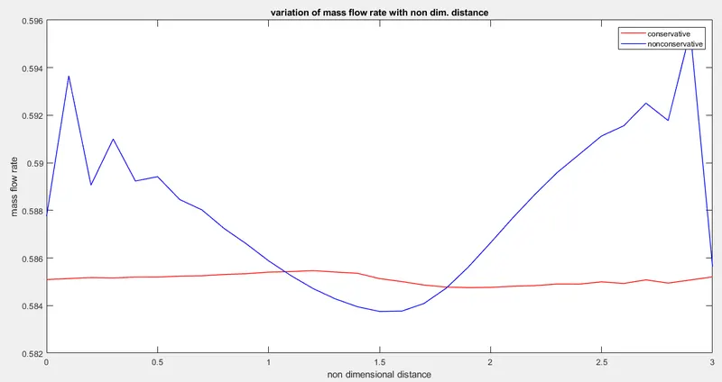
n=31

variation of mass flow rate with non dimensional distance for conservative and nonconservative method

conservative time=3.1360sec

non-conservative time=1.8217sec

n=61

variation of mass flow rate with non dimensional distance for conservative and nonconservative method

conservative time=3.2739sec

non-conservative time=1.9492sec

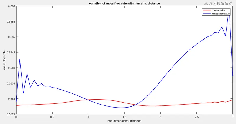
This graph is the comparison between conservative and non-conservative mass flow rate through the nozzle.The time taken for conservative approach is more than non-conservative approach.More fluctuation is seen in the non-conservative approach,as the control volume taken into consideration for analysis is moving with the flow,so the primitive variables will be well studied.As the case for conservative approach, the control volume taken for analysis is fixed in space.so, it is well suited for flux terms and is giving steady results.

The time taken for non-conservative approach is 1.8217 for 31 grid points ,1.9492 for 61 grid points. As the grid points increases the time taken also increases but not that much high.so,it is showing grid independence criteria.

n=31

mass flow rate for different time step for nonconservative method

n=61

mass flow rate for different time step for nonconservative method

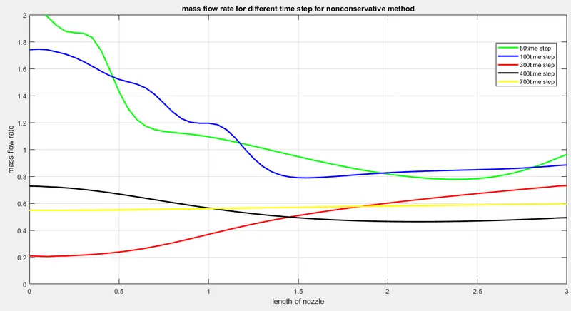
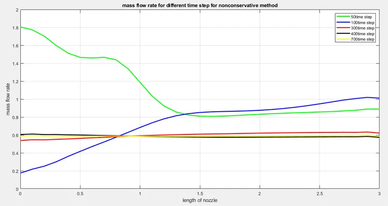
In this figure, the mass flow inside the nozzle varies at different time step .The variation converges to a steady state solution at time step greater than 300time step. The 400 and 700 time step shown in figure as black and yellow ,converges to the steady state solution faster.

n=31

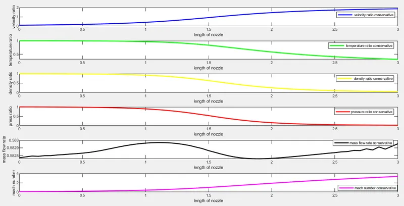
variation of flow variables inside the nozzle for conservative method

n=61

variation of flow variables inside the nozzle for conservative method

N=31

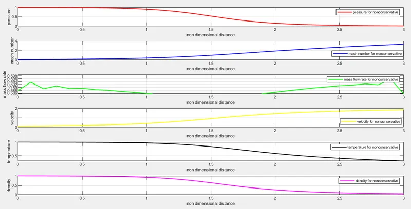
variation of flow variables inside the nozzle for non-conservative method

N=61

variation of flow variables inside the nozzle for non-conservative method

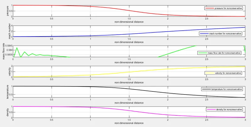
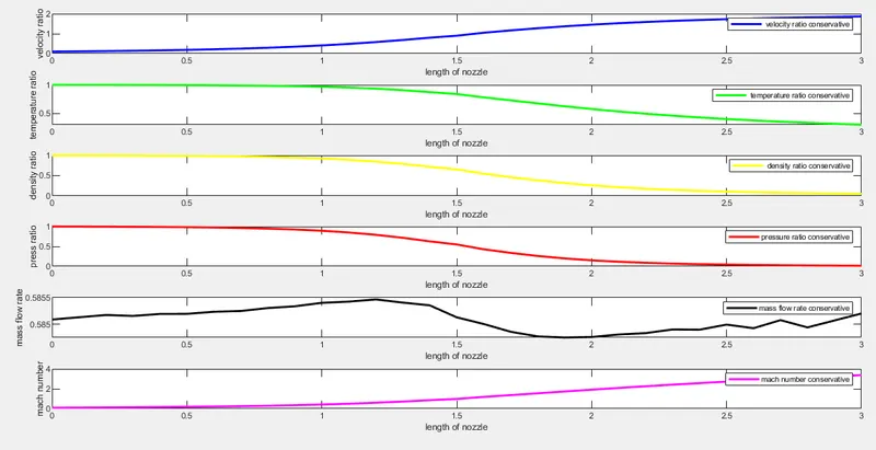
• This figure shows the variation of flow field variables inside the nozzle. The velocity profile shown here is correct as it increases as it passes through the supersonic region.
• As the fluid is passing through the divergent part of nozzle the temperature and pressure decreases as shown in figure.

n=31

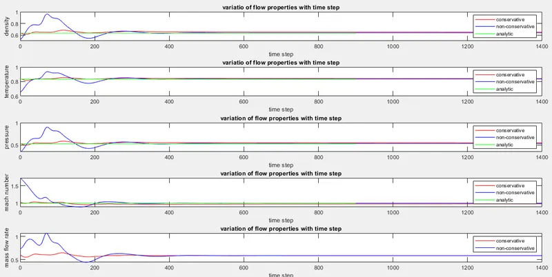
variation of flow variables inside the nozzle at different time step

N=61

variation of flow variables inside the nozzle at different time step

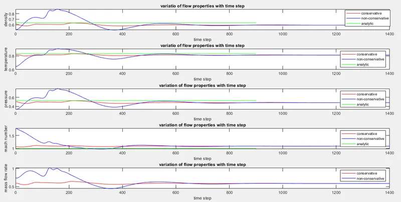
• The above fig shows the variation of flow variables inside the nozzle at varying time step for conservative,nonconservative and analytic solution. The values of flow field variables are converging to analytic solution at time steps nearly equal to 400 to 500 steps.
• The conservative approach reaches the analytic solution at 300 to 350 time steps.

• The conservative form does a better job of preserving mass throughout the flow field.
• For flux variables ,conservation form produces more accurate results.
• For primitive variables(T,P,rho,V )non-conservation form produces more accurate results.
• we are getting smaller residuals in non-conservation form.

Non-Conservative

No. of grids density Temperature pressure mach number

31 0.6387 0.8356 0.5342 0.999

61 0.5940 0.8121 0.4824 1.082

Conservative

No. of grids density Temperature pressure mach number

31 0.6524 0.8411 0.5487 0.978

61 0.5929 0.8109 0.4807 1.0858