Week 5.1 - Mid term project - Solving the steady and unsteady 2D heat conduction problem
AIM: Solving the steady state 2-D heat conduction equation using point iterative techniques .
GIVEN: The Boundary conditions for the problem are as follows;
Top Boundary = 600 K
Bottom Boundary = 900 K
Left Boundary = 400 K
Right Boundary = 800 K
we will implement the following methods for solving implicit equations :
1. Jacobi
2. Gauss-seidel
3. Successive over-relaxation
The absolute error criteria is 1e-4.(tol=1e-4)
- There are two types of solution methods for the linear algebraic equations of the form [A][X]=[B],
- The first kind include direct methods such as gauss-elimination,Thomas-algorithm,Chelosky method etc.
- The second kind includes iterative methods such as Jacobi iteration,Gauss-siedal iteration,successive over relaxation,ADI and so on.
- disadvantage of direct methods:
- more time consuming.
- susceptible to round-off errors.
general heat conduction equation:
`(d^2T)/(dx^2)+(d^2T)/(dy^2)+(d^2T)/(dz^2)+q_g/k=1/alpha*(dT)/dt`
where the property alpha=k/(rho*Cp) is the thermal diffusivity of the material.
q_g=heat generation
steady state equation having no heat generation
`(d^2T)/dx^2 +(d^2T)/dy^2 =0`
(T_L-2*T_P +T_R)/dx^2 +(T_T-2*T_P+T_B)/dy^2 =0``
`(2*T_P)/dx^2 +(2*T_P)/dy^2 =(T_L+T_R)/(dx^2)+(T_T+T_B)/(dy^2)`
T_P=((T_L+T_R)/(dx^2)+(T_T+T_B)/(dy^2))/k`
where k=`2*(dx^2 +dy^2)/(dx^2*dy^2)`
- Jacobi method: In this method ,the unknown variable(in this case temp.) at each grid point is solved in terms of the initial guess values or previously computed values.
- Gauss-seidal method: In this method the current values of the dependant variables are used to compute neighbouring points as soon as they are available.This will increase the convergence rate.
JACOBI METHOD (STEADY STATE)


steady state heat_conduction_problem
clear all
close all
clc
%steady_state_equation
% dT^2/dx^2+dT^2/dy^2=0
nx=10;
ny=10;
L=1;
x=linspace(0,L,nx);
dx=x(2)-x(1);
y=linspace(0,L,ny);
dy=dx;

T=300*ones(nx,ny);
T(:,1)=400;
T(1,:)=600;
T(10,:)=900;
T(:,end)=800;

T(1,1)=500;
T(1,end)=700;
T(10,1)=650;
T(10,10)=850;
%initialise
T_old=T;
k=(2*(dx^2+dy^2)/((dx^2)*(dy^2)));

iterative_solver=1
error=20;
%jacobi_method
tol=1e-4;
if iterative_solver==1
    tic
    jacobi_iteration=1;
    while (error>tol)
        for i=2:nx-1
            for j=2:ny-1
                Term1=(T_old(i-1,j)+T_old(i+1,j))/(k*dx^2);
                Term2=(T_old(i,j+1)+T_old(i,j-1))/(k*dy^2);
                T(i,j)=Term1+Term2;
            end
        end
        error=max(max(abs(T-T_old)));
        jacobi_iteration=jacobi_iteration+1;
        T_old=T;

    %plotting
    figure(1)
    [x1,y1]=contourf(x,y,T);
    set(gca,'YDIR','reverse')
    colorbar
    colormap(jet);
    clabel(x1,y1);
    xlabel('x-axis')
    ylabel('y-axis')
    text_title=sprintf('temperature_jacobi_iteration=%d',jacobi_iteration);
    title(text_title)
    pause(0.3)
    end
time_jacobi=toc;
end


.............................................*****.....................


GAUSS-SEIDAL


T_old=T;
k=(2*(dx^2+dy^2)/((dx^2)*(dy^2)));
error=20;
tol=1e-4;
iterative_solver=2
if iterative_solver==2
    tic
    gs_iteration=1;
    while (error>tol)
        for i=2:nx-1
            for j=2:ny-1
                term(3)=(T_old(i+1,j)+T(i-1,j))/dx^2;
                term(4)=(T_old(i,j+1)+T(i,j-1))/dy^2;
                T(i,j)=(term(3)+term(4))/(k);
            end
        end

        error=max(max(abs(T-T_old)));
        gs_iteration=gs_iteration+1;
            T_old=T;

    %plotting
    figure(2)
    [x1,y1]=contourf(x,y,T);
    set(gca,'YDIR','reverse')
    colormap(jet);
    clabel(x1,y1)
    xlabel('x-axis')
    ylabel('y-axis')

    text_title=sprintf('temperature_gs_iteration=%d',gs_iteration);
    title(text_title)
    pause(0.3)
    end
time_gs=toc;
end

..................................*********................................

SOR (STEADY STATE)

%initialise
T_old=T;
k=(2*(dx^2+dy^2)/((dx^2)*(dy^2)));
error=20;
tol=1e-4;
iterative_solver=3
if iterative_solver==3
    tic
    w=1.3;
    sor_iteration=1;
    while (error>tol)
        for i=2:nx-1
            for j=2:ny-1
                T(i,j)=w*(((T_old(i+1,j)+T(i-1,j))/(dx^2)+(T_old(i,j+1)+T(i,j-1))/(dy^2)))/(k)+(1-w)*T_old(i,j);
            end
        end
        error=max(max(abs(T-T_old)));
        sor_iteration=sor_iteration+1;
        T_old=T;

    %plotting
    figure(3)
    [x1,y1]=contourf(x,y,T);
    set(gca,'YDIR','reverse');
    colormap(jet);
    clabel(x1,y1);
    xlabel('x-axis')
    ylabel('y-axis')
    text_title=sprintf('temperature_sor_iteration=%d',sor_iteration);
    title(text_title)
    pause(0.03)
    end
time_sor=toc;
end
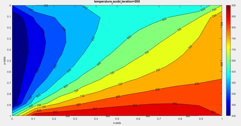
jacobi_iteration=208
jacobi_time=118.7028 sec
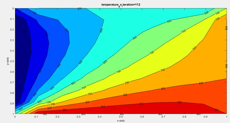
gs_iteration=112
gs_time=43.4149 sec
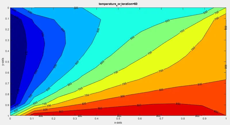
sor_iteration=60
sor_time=10.7949
- For explicit method, the temperature value at next time-step is calculated by taking the values of temperature at previous time step.The thermal diffusivity(alpha) is taken as 1e-2, for faster convergence.Also,it defines conduction taking at a faster rate.
Explicit Method


clear all
close all
clc
% explicit scheme

nx=10;
ny=10;
L=1;
x=linspace(0,L,nx);
dx=x(2)-x(1);
y=linspace(0,L,ny);
dy=dx;
%initialise
T=300*ones(nx,ny);
T(:,1)=400;
T(1,:)=600;
T(10,:)=900;
T(:,end)=800;

T(1,1)=500;
T(1,end)=700;
T(10,1)=650;
T(10,10)=850;
% tol=1e-4;
% error=10;
alpha=1e-2;
dt=0.01;
k1=(alpha*dt)/dx^2;
k2=(alpha*dt)/dy^2;
% T_prev=T;
T_old=T;

    tic
    for k=1:2000

        for i=2:nx-1
            for j=2:ny-1
            T(i,j)=T_old(i,j)+k1*(T_old(i-1,j)-2*T_old(i,j)+T_old(i+1,j))+k2*(T_old(i,j+1)-2*T_old(i,j)+T_old(i,j-1));
        end
    end
    T_old=T;
    end
     %plotting
    figure(1)
    [x1,y1]=contourf(x,y,T);
    set(gca,'YDIR','reverse')
    colorbar
    colormap(jet);
    clabel(x1,y1);
    xlabel('x-axis')
    ylabel('y-axis')
%     text_title=sprintf('temperature_jacobi_iteration=%d',jacobi_iteration);
%     title(text_title)
    pause(0.3)
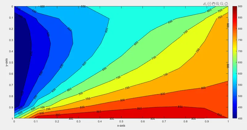
expilcit_iteration=1700 time step
explicit_time=1.4705 sec
TRANSIENT STATE ANALYSIS
In this analysis ,we mainly focused on calcuating the temperature value at time step (n+1) by taking the value of temperature at (n+1) time_step.
`(d^2T)/(dx^2)+(d^2T)/(d^y)-(alpha)*(dT)/dt=0`
discretizing the above equation:
`T_(i,j)^(n+1) =T_(i,j)^n +(alpha)*(deltat)(((T_(i+1,j)^(n+1)-2*T_(i,j)^(n+1)+T_(i-1,j)^(n+1))/(deltax^2)+(T_(i,j+1)^(n+1)-2*T_(i,j)^(n+1)+T_(i,j-1)^(n+1))/(deltay^2))^(n+1)`
let, `T_(i,j)^n=T_P`
`T_(i+1,j)^(n+1)=T_R`
`T_(i-1,j)^(n+1)=T_L`
`T_(i,j+1)^(n+1)=T_T`
`T_(i,j-1)^(n+1)=T_B`
`T_P^(n+1)=T_P^(n)+k1*(T_R-2*T_P+T_L)^(n+1)+k2*(T_T-2*T_P+T_B)^(n+1)`
where k1=`alpha*(deltat)/(deltax^2)` and k2=`alpha*(deltat)/(deltay^2)`
again rearraging the terms we get:
`T_P^(n+1)*k=T_P^n +k1*T_L^(n+1)+k1*T_R^(n+1)+k2*T_T^(n+1)+k2*T_B^(n+1)`
where k=`1+2k1+2k2`
`T_P^(n+1)=(T_P^(n))/k+(k1*(T_L+T_R)^(n+1)+k2*(T_T+T_B)^(n+1))/k`
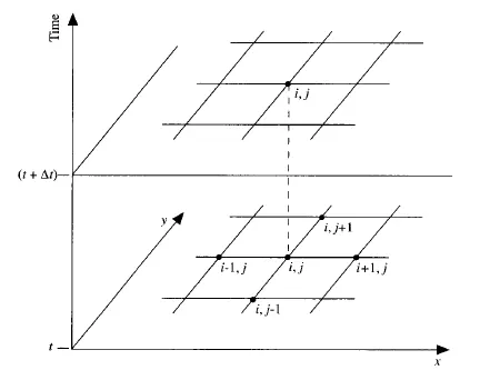
fig. A schematic of the grid for time marching( John anderson)
JACOBI METHOD

%Transient_heat_conduction_problem
clear all
close all
clc
%Transient_state_equation
% dT^2/dx^2+dT^2/dy^2-(alpha)*dT/dt=0
nx=10;
ny=10;
L=1;
x=linspace(0,L,nx);
dx=x(2)-x(1);
y=linspace(0,L,ny);
dy=dx;

T=300*ones(nx,ny);
T(:,1)=400;
T(1,:)=600;
T(10,:)=900;
T(:,end)=800;

T(1,1)=500;
T(1,end)=700;
T(10,1)=650;
T(10,10)=850;
%initialise
T_old=T;
T_prev=T;
alpha=1.2;
dt=0.01;
k1=(alpha*dt)/(dx^2);
k2=(alpha*dt)/(dy^2);
error=10;
tol=1e-4;
iterative_solver=1
if (iterative_solver==1)
    tic
    jacobi_iter=1;
    term1=(1+(2*k1)+(2*k2))^-(1);
    term2=k1*term1;
    term3=k2*term1;
%     H=T_old(i+1,j)+T_old(i-1,j);
%     V=T_old(i,j+1)+T_old(i,j-1);
    for k=1:1700
        error=10;
        while(error>tol)
        for i=2:nx-1
            for j=2:ny-1
                H=T_old(i+1,j)+T_old(i-1,j);
                V=T_old(i,j+1)+T_old(i,j-1);
                T(i,j)=(T_prev(i,j)*term1+(H*term2)+V*term3);
            end
        end
        error=max(max(abs(T-T_old)));
        jacobi_iter=jacobi_iter+1;
        T_old=T;
        end
    T_prev=T;
    end
    %plotting
    figure(3)
    [x1,y1]=contourf(x,y,T);
    set(gca,'YDIR','reverse');
    colormap(jet);
    clabel(x1,y1);
    xlabel('x-axis')
    ylabel('y-axis')
    text_title=sprintf('temperature_at_time_step-%d_jacobi_iteration=%d',k,jacobi_iter);
    title(text_title)
    pause(0.03)
    time_jacobi=toc;
end
GAUSS-SEIDAL METHOD
%initialise
T_old=T;
T_prev=T;
alpha=1.2;
dt=0.01;
k1=(alpha*dt)/(dx^2);
k2=(alpha*dt)/(dy^2);
error=10;
tol=1e-4;
iterative_solver=2
if (iterative_solver==2)
    tic
    gs_iter=1;
    term1=(1+(2*k1)+(2*k2))^-(1);
    term2=k1*term1;
    term3=k2*term1;
%     H=T_old(i+1,j)+T(i-1,j);
%     V=T_old(i,j+1)+T(i,j-1);
    for k=1:1700
        error=10;
        while (error>tol)
        for i=2:nx-1
            for j=2:ny-1
                H=T_old(i+1,j)+T(i-1,j);
                V=T_old(i,j+1)+T(i,j-1);
                T(i,j)=(T_prev(i,j)*term1+(H*term2)+V*term3);
            end
        end
        error=max(max(abs(T-T_old)));
        gs_iter=gs_iter+1;
        T_old=T;
        end
    T_prev=T;
    end
    %plotting
    figure(3)
    [x1,y1]=contourf(x,y,T);
    set(gca,'YDIR','reverse');
    colormap(jet);
    clabel(x1,y1);
    xlabel('x-axis')
    ylabel('y-axis')
    text_title=sprintf('temperature_at_time_step-%d_gs_iteration=%d',k,gs_iter);
    title(text_title)
    pause(0.03)
    time_gs=toc;
end
SOR METHOD
%initialise
T_old=T;
T_prev=T;
alpha=1.2;
dt=0.01;
k1=(alpha*dt)/(dx^2);
k2=(alpha*dt)/(dy^2);
k=(2*(dx^2+dy^2)/((dx^2)*(dy^2)));
error=10;
tol=1e-4;
iterative_solver=3
if (iterative_solver==3)
    tic
    w=1.25;
    sor_iter=1;
    term1=(1+(2*k1)+(2*k2))^-(1);
    term2=k1*term1;
    term3=k2*term1;
%     H=T_old(i+1,j)+T(i-1,j);
%     V=T_old(i,j+1)+T(i,j-1);
    for k=1:1700
        error=10;
        while (error>tol)
        for i=2:nx-1
            for j=2:ny-1
                H=T_old(i+1,j)+T(i-1,j);
                V=T_old(i,j+1)+T(i,j-1);
                T(i,j)=((1-w)*T_prev(i,j))+w*((T_prev(i,j)*term1+(H*term2)+V*term3));
            end
        end
        error=max(max(abs(T-T_old)));
        sor_iter=sor_iter+1;
        T_old=T;
        end
    T_prev=T;
    end
    %plotting
    figure(3)
    [x1,y1]=contourf(x,y,T);
    set(gca,'YDIR','reverse');
    colormap(jet);
    clabel(x1,y1);
    xlabel('x-axis')
    ylabel('y-axis')
    text_title=sprintf('temperature at time step-%d sor iteration=%d',k,sor_iter);
    title(text_title)
    pause(0.03)
    time_sor=toc;
end
implicit_jacobi_iteration=3050 at time step=1700
time_jacobi=1.1828 sec
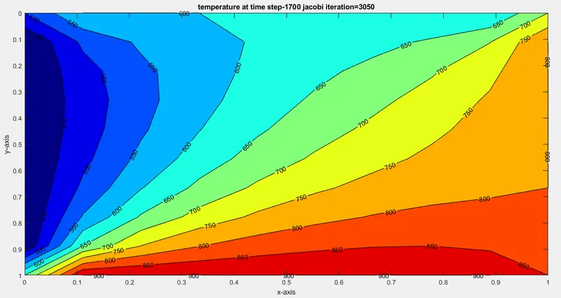
implicit_gs_iteration=2524 at time step=1700
time_gs=1.1162 sec
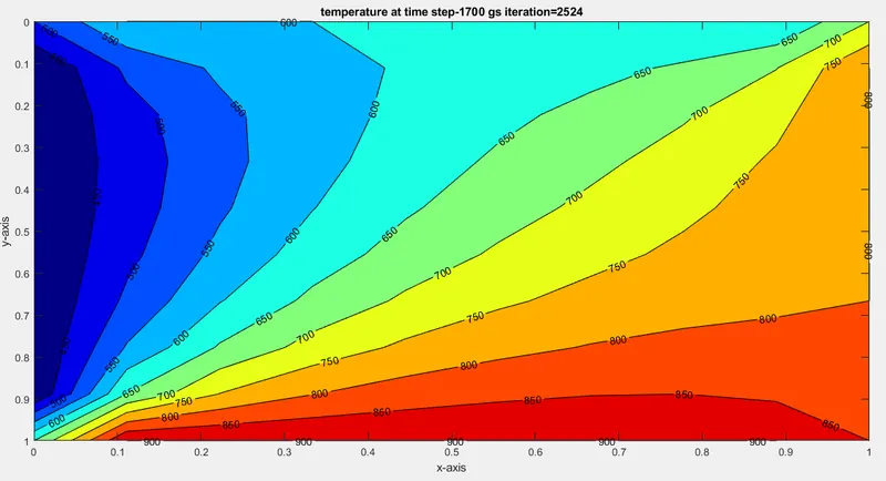
implicit_sor_iteration=2035,time_step=1700
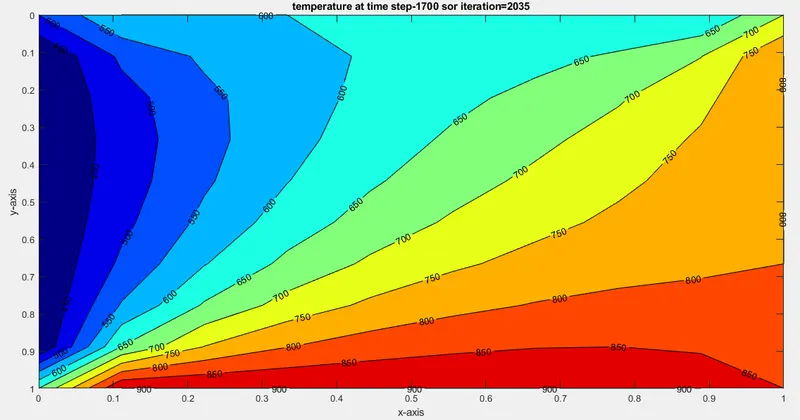
conclusion:
- As we have seen in the above graph that for Jacobi_iteration whether it is steady or transient the time taken for computation is large as compared to Gauss-seidal and sor method.
- For explicit method ,we found that the time taken for 1700 time step iteration is more than impcit method.Implicit SOR is taking less time than implicit jacobi and implicit gauss-seidal.