Week 7 - Minor Project
Aim
To simulate subsonic and supersonic flow over the NACA 0012 airfoil at various angles of attack (5,10, and 15 degrees) and compare the lift and drag coefficients.
Introduction
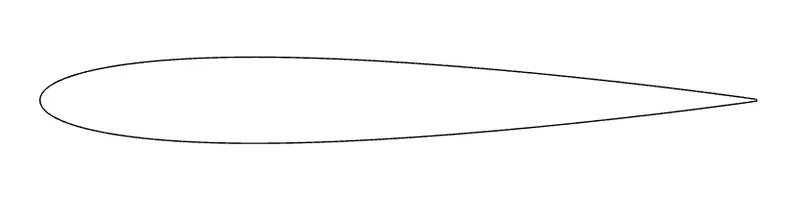
The NACA 0012 airfoil is a symmetric airfoil with a maximum thickness of 12% of the chord and can be seen in the image below.
The forces acting on the airfoil are illustrated in the schematic shown below.
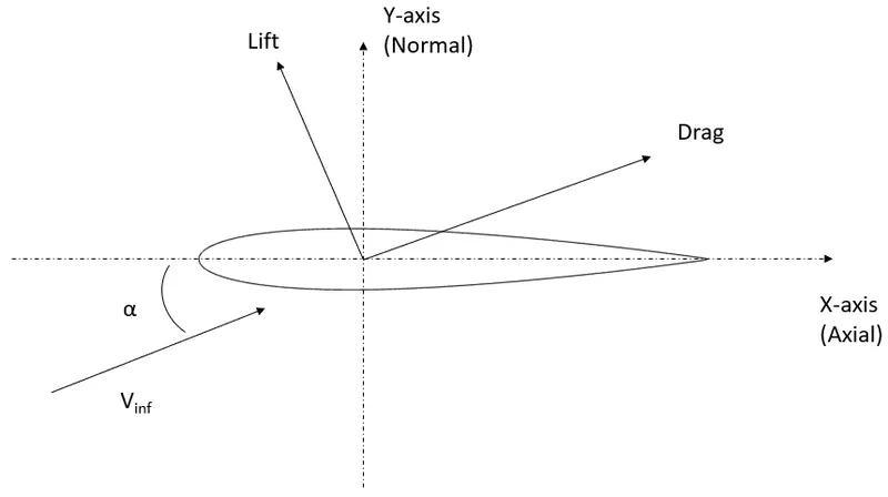
From the above image, it is possible to resolve the lift and drag vectors as components of X (Axial) and Y (Normal)
vectors as:
Drag = Xcos`alpha` + Ysin`alpha`
Lift = Ycos`alpha` - Xsin`alpha`
Where, `alpha` is the angle of attack.
With the lift and drag forces estimated, the respective coefficients can be estimated as follows:
`Cl = L/((1/2)rho V^2 c)`
`Cd = D/((1/2)rho V^2 c)`
Where,
`rho` - Density of the fluid [`kgm^-3`]
V - Free stream velocity [`ms^-1`]
c - chord length of the airfoil [m]
L/D - Lift/Drag forces [N]
Method
Domain and Mesh
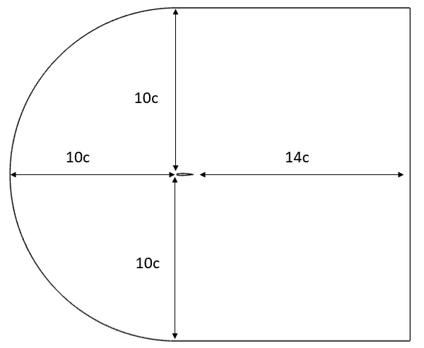
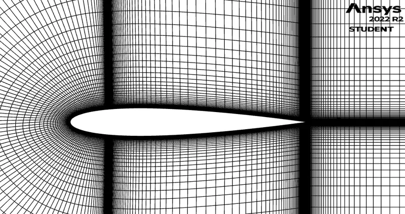
All simulations will be conducted in 2-dimensions as only the flow over the airfoil is of interest. The domain sizings around the airfoil can be seen in the schematic below.
The subsonic case will be run at Mach = 0.2
The supersonic case will be run at Mach = 2.0
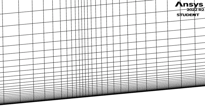
Using the yplus calculator to estimate the required first layer height (with air at default properties) for a yplus = 1,
First layer height of subsonic case = 5.5e-6 m
First layer height of supersonic case = 6.52e-7 m
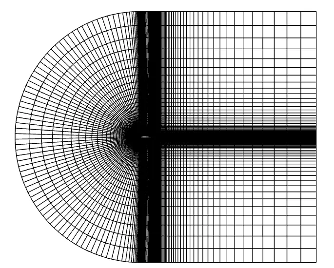
The resulting mesh with the appropriate first layer height can be seen below.
Subsonic case:
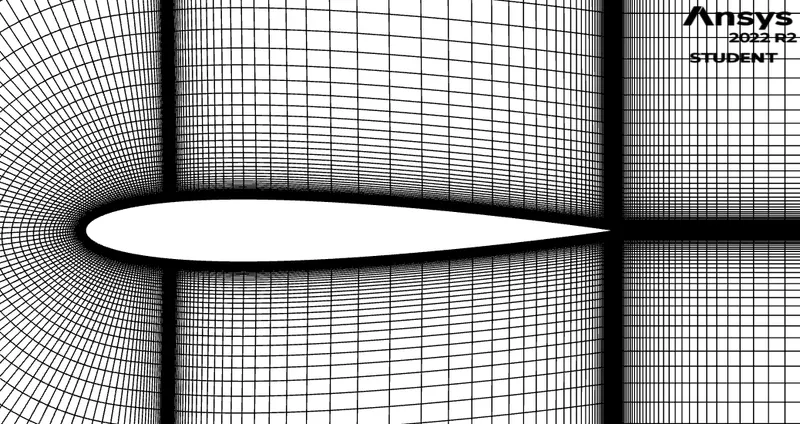
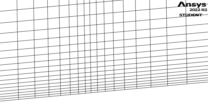
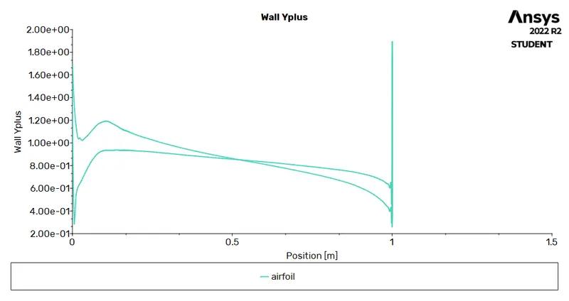
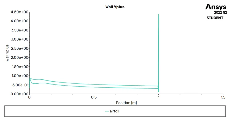
The image below shows the typical yplus plot over the airfoil at Mach 0.2.
Supersonic case:
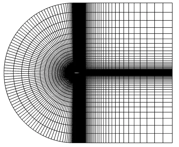
The image below shows the typical yplus plot over the airfoil at Mach 2.0.
CFD Setup
All simulations were conducted on ANSYS Fluent 2022R2. Air was used as the fluid with density estimated using the ideal gas formulation. All the frontal domain surfaces were set to a pressure far-field with a pressure outlet condition at the rear. The Mach number was set to 0.2 for the subsonic case and 2.0 for the supersonic case. The X and Y components of the flow were input to Fluent using the following expression,
X-component of flow direction= `cos(alpha*(pi/180))`
Y-component of flow direction= `sin(alpha*(pi/180))`
where `alpha` is the angle of attack for the various cases.
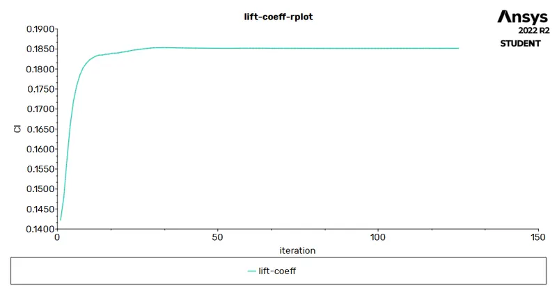
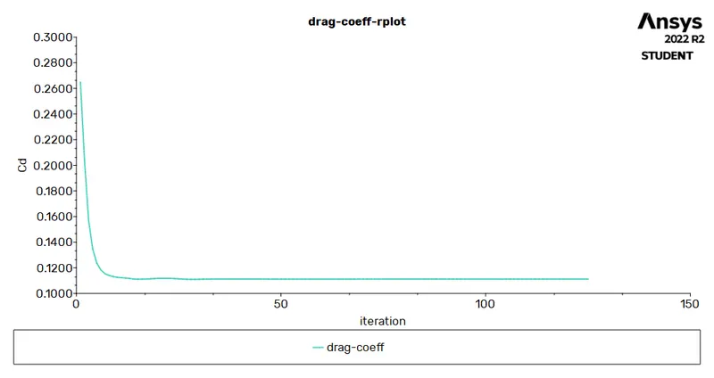
The steady-state pressure-based PV coupled solver was used to discretize the flow parameters. Turbulence in the flow was predicted using the one-equation Spalart-Allmaras model. The second-order scheme was used to estimate the pressure, the second-order upwind scheme was used to estimate momentum, energy, and turbulence parameters. The solution was initialized by a standard initialization followed by an FMG initialization to quicken convergence. The simulation was run with pseudo transient time stepping with an automatic global conservative length scale. Convergence was checked by scaled residuals achieving 1e-3 units and the change in Cl and Cd not exceeding 1e-3 units across iterations. The simulations typically converged within 150 iterations.
Results
Subsonic Case:
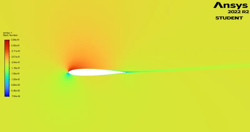
Case 1: `alpha` =5, M = 0.2
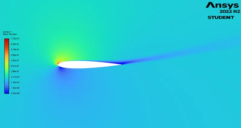
The image below shows the Mach number distribution over the airfoil.
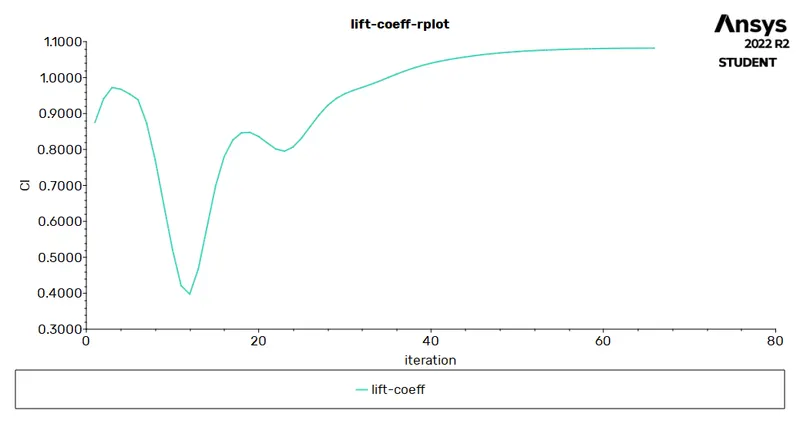
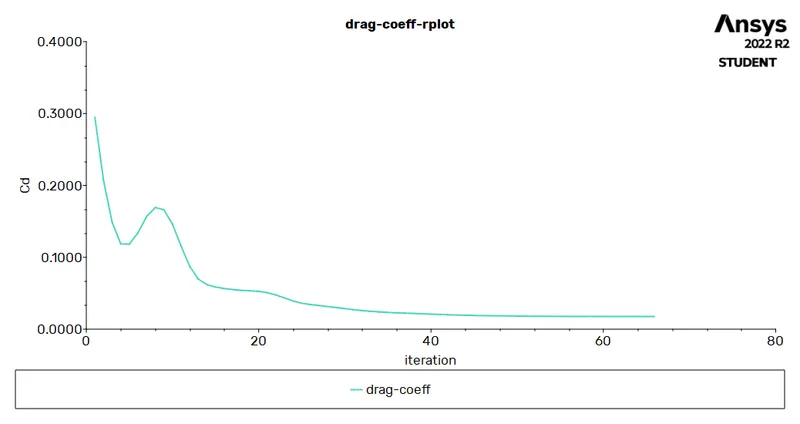
The plots below show the lift and drag convergence
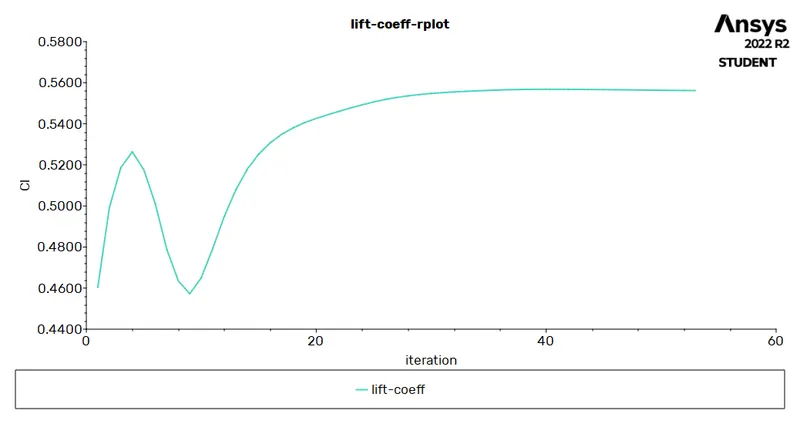
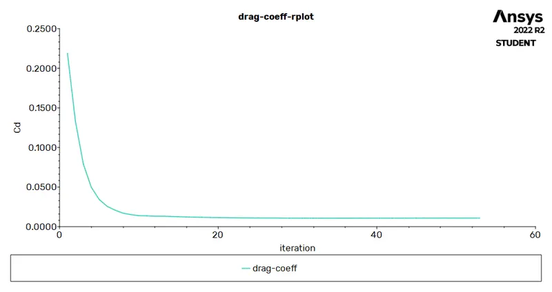
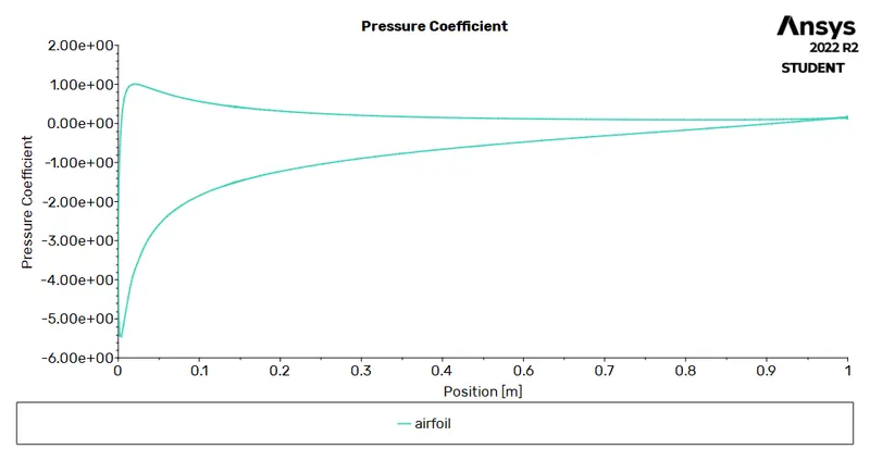
The plot below shows the distribution of the pressure coefficient on the surface of the airfoil.
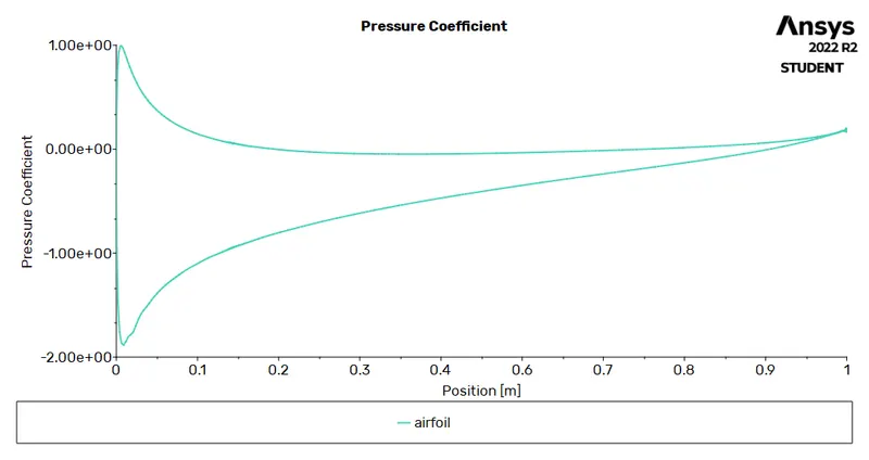
Case 2: `alpha` =10, M = 0.2
The image below shows the Mach number distribution over the airfoil.
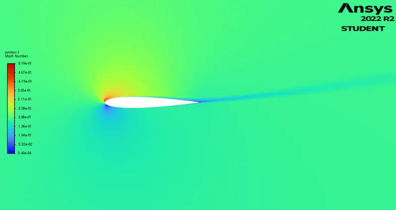
The plots below show the lift and drag convergence
The plot below shows the distribution of the pressure coefficient on the surface of the airfoil.
Case 3: `alpha` =15, M = 0.2
The image below shows the Mach number distribution over the airfoil.
The plots below show the lift and drag convergence
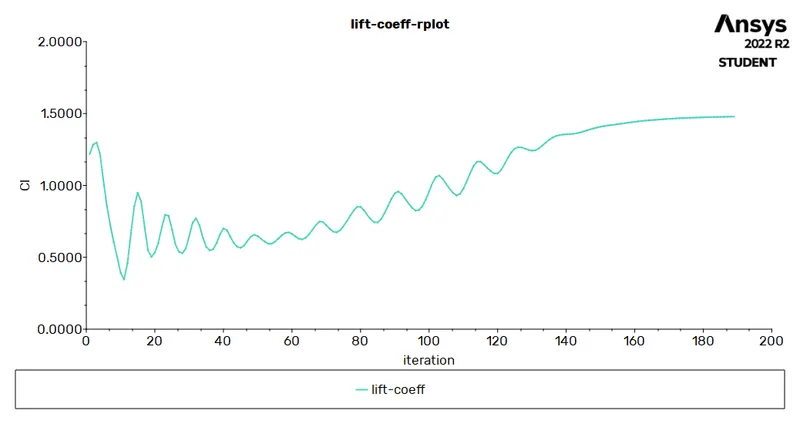
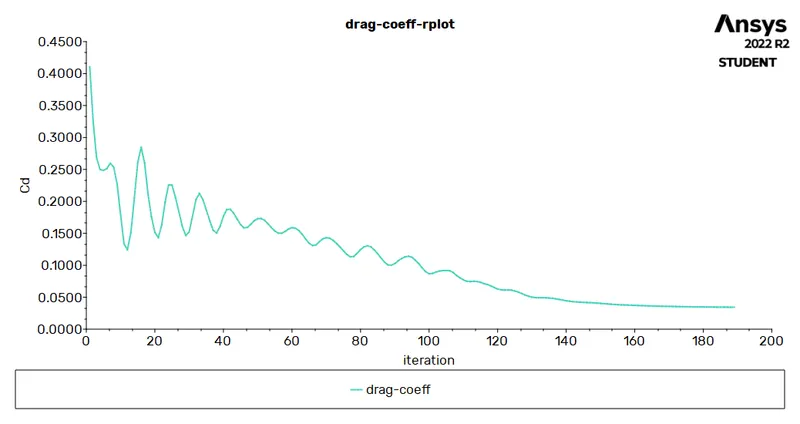
The plot below shows the distribution of the pressure coefficient on the surface of the airfoil.
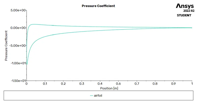
Supersonic Case:
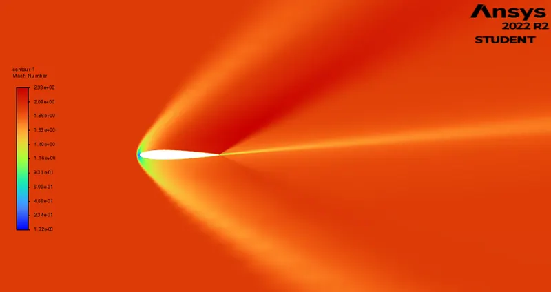
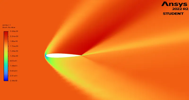
Case 1: `alpha` =5, M = 2.0
The image below shows the Mach number distribution over the airfoil.
The plots below show the lift and drag convergence
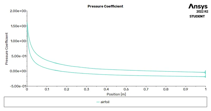
The plot below shows the distribution of the pressure coefficient on the surface of the airfoil.
Case 2: `alpha` =10, M = 2.0
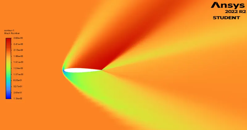
The image below shows the Mach number distribution over the airfoil.
The plots below show the lift and drag convergence
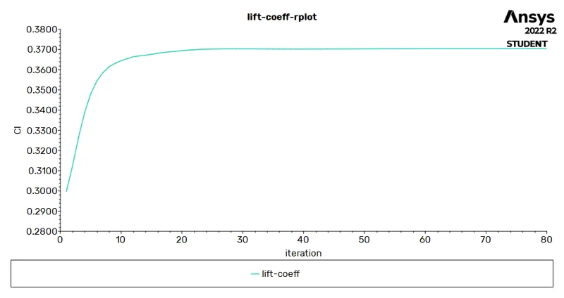
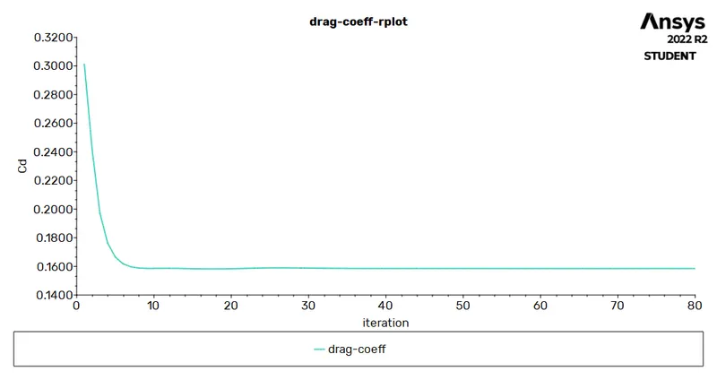
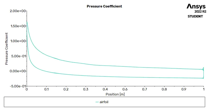
The plot below shows the distribution of the pressure coefficient on the surface of the airfoil.
Case 3: `alpha` =15, M = 2.0
The image below shows the Mach number distribution over the airfoil.
The plots below show the lift and drag convergence
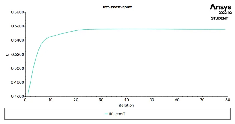
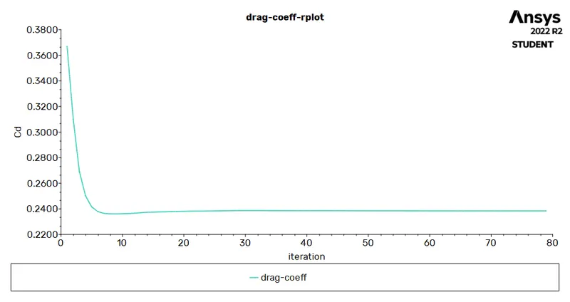
The plot below shows the distribution of the pressure coefficient on the surface of the airfoil.
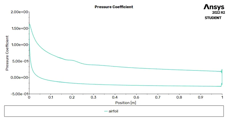
The Lift and Drag coefficients for all the simulations are tabulated below.
| Mach 0.2 | Mach 2.0 | |||
| Angle of Attack [degrees] | CL | CD | CL | CD |
| 5 | 0.556 | 0.011 | 0.185 | 0.111 |
| 10 | 1.082 | 0.018 | 0.370 | 0.159 |
| 15 | 1.478 | 0.034 | 0.555 | 0.238 |
From the above table, it can be seen that the lift and drag coefficients increase with increasing angles of attack for both the subsonic and supersonic cases. The drag coefficient is much higher in the supersonic case and can be attributed to the wave drag created by the shockwaves. The lift coefficient is also drastically reduced in the supersonic case due to the generation of shockwaves.
Conclusion
Flow simulations were performed over the NACA 0012 airfoil at various angles attack in both the subsonic and supersonic Mach regimes and the lift and drag coefficients were estimated. Both Mach regimes showed an increase in lift and drag coefficients with increasing angle of attack. The supersonic case however consistently showed a reduced lift coefficient and increased drag coefficient compared to the subsonic case. This disparity was attributed to the formation of shockwaves in the flow field in the supersonic case.