Week 7 Gear

For this challenge, you have to perform the four simulations in the Gearbox and then you have to compare the results among all the four cases.

Part 1:

1. 20% Immersion, Fluid - Engine oil.
2. 30% Immersion, Fluid- Engine oil.
3. 20% Immersion,Fluid-n-heptane (c7h16).
4. 30% Immersion,Fluid-n-heptane (c7h16).

Part 2:

1. What is Dynamic meshing? Give some other examples where dynamic meshing can be used.
2. What is the fluid Sloshing effect? Discuss whether the sloshing effect is good or bad? Explain.
3. What is the use of UDF?
4. Discuss the common errors that occurred in the simulation. A] 'Dynamic mesh failed' error. B] 'Negative cell volume detected' error.

Objective:

With regard to this challenge,

• We will talk about what dynamic meshing is and give some other examples of how it can be used.
• We then debate the pros and cons of the sloshing effect in fluids.
• Following that, we will talk about why UDF is used.
• The next step is the most important one, which is that we are going to run four simulations within the Gearbox, and then we are going to compare the outcomes of those simulations across all four scenarios.
• The four scenarios are as follows:

1. 20% Immersion in Fluid, Engine oil was used.
2. 30% immersion in the fluid, which was engine oil.
3. 20% Immersion,Fluid-n-heptane (c7h16).
4. 30% Immersion,Fluid-n-heptane (c7h16).

In the end, we are going to talk about the typical mistakes that will take place during the simulation. An error that reads "Dynamic mesh failed." and 'Negative cell volume detected' error.

In the beginning...

This method of analysis is very common in industry, and its purpose is to determine whether or not a particular gearbox setup with a given lubricant is able to reach all of the gear's teeth adequately, as well as whether or not the gear achieves adequate performance.

Let's begin by discussing some theory concerning dynamic meshing, fluid sloshing, and UDFs.

The use of dynamic meshing:

The dynamic mesh model enables you to modify the boundaries of a cell zone in relation to those of other cell zone boundaries, and it also enables you to adjust the mesh in accordance with these modifications. Both rigid movement (in the form of linear or rotational motion) and deformation of the boundaries with respect to one another are both possible.

Boundaries can move either rigidly, like pistons in an engine cylinder, or deformably, like a balloon's elastic wall during inflation or a flexible artery wall in response to a pressure pulse from the heart. In either scenario, the nodes that define the cells in the domain need to be updated as a function of time, and as a result, the solutions provided by the dynamic mesh are inherently unstable.

The sliding mesh is a significant subtype of the dynamic mesh motion that occurs when all of the boundaries and the cells of a given mesh zone move together in a rigid-body motion. This is an important aspect of the sliding mesh. In this scenario, the nodes of the mesh move in space (relative to the global coordinates that remain constant), but the cells that are defined by the nodes do not change shape. In addition, mesh zones that are moving adjacent to one another can be linked together through the use of one or more non-conformal interfaces. The non-conformal interfaces can be dynamically updated as the meshes move so that fluid can move from one zone to another as long as the interfaces continue to remain in contact with one another (that is, "slide" along a common overlap boundary at the interface).

ANSYS Fluent's dynamic mesh model can be used to model flows in situations where the shape of the domain is changing over the course of the simulation as a result of motion on the domain boundaries. The dynamic mesh model can be used to analyse single-phase flows as well as multiphase flows (and multi-species flows). At each time step, ANSYS Fluent will automatically handle the update of the volume mesh based on the new positions of the boundaries. This process is completely hands-free. In order to make use of the dynamic mesh model, it is necessary for you to supply a starting volume mesh as well as a description of the movement of any moving zones contained within the model. You are able to describe motion in ANSYS Fluent by employing boundary profiles, user-defined functions (UDFs), or the six degrees of freedom solver.

ANSYS Fluent anticipates that the motion description will be specified either on the face zones or the cell zones. If the model has regions that move and regions that do not move, you will need to identify these regions in the starting volume mesh that you generate by grouping them into the face or cell zones that correspond to the moving and non-moving regions, respectively. Additionally, in the starting volume mesh, regions that are deforming as a result of motion on their neighbouring regions need to be grouped together into distinct zones. There is no requirement that the boundaries between the various regions conform to any particular pattern. To connect the different zones that make up the final model, you can make use of the non-conformal or sliding interface capability that is available in ANSYS Fluent.

Within ANSYS Fluent, there are three different groups of mesh motion methods that can be used to update the volume mesh in the deforming regions that are subject to the motion that is defined at the boundaries.

1. Smoothing Methods.
2. Dynamic Layering.
3. Remeshing Methods.

1. Smoothing Methods:

The internal nodes of the mesh move when smoothing is used to alter the mesh of a zone that has a moving and/or deforming boundary, but the total number of nodes and the connection between them does not change. The movement of the boundary is effectively "absorbed" by the interior nodes in this manner.

2. Dynamic layering:

The dynamic layering approach can be used to split or combine cells near to any moving border if the prerequisites are met:

Despite the fact that the cell zone itself may contain a variety of different cell shapes, all cells that are next to the moving face zone are either wedges or hexahedra (quadrilaterals in 2D).
Except in cases when sliding interfaces are used, the cell layers have to be entirely surrounded by face zones that only expose one side.

3. Remeshing Methods:

If just mesh smoothing is employed, the cell quality may decline or the cells may become degenerate if the boundary displacement is substantial in comparison to the local cell sizes. This may occur if only mesh smoothing is used. Because of this, the mesh will become invalid (for example, it will result in negative cell volumes), and as a consequence, there will be problems with convergence when the solution is updated to the next time step.
ANSYS Fluent agglomerates cells that do not comply with the skewness or size criterion and then locally remeshes the agglomerated cells or faces in order to get around this issue. In the event that the newly added cells or faces pass the skewness test, the mesh is then locally modified to include the newly added cells (with the solution interpolated from the old cells). If this does not happen, the new cells are thrown away while the old cells are preserved.
Local cell remeshing, zone remeshing, local face remeshing (only for 3D flows), face region remeshing, and 2.5D surface remeshing are some of the remeshing methods that are included in ANSYS Fluent (for 3D flows only).

Fluid Sloshing effect :

When discussing fluid dynamics, the term "slosh" is used to describe the flow of liquid within a different substance (which is, typically, also undergoing motion).
A slosh dynamics problem exists when the liquid's dynamics interact with the container's dynamics to dramatically modify the system dynamics, yet this requires the liquid to have a free surface. Notable measures are propellant slosh in spacecraft tanks and rockets (particularly higher stages), as well as the free surface effect (cargo slosh) in ships and trucks transporting liquids. Both of these types of slosh can occur when liquids are being moved (for example oil and gasoline). But it has become common to say "fuel slosh" when liquid moves in a tank that is full to the top and has no free surface.
Such motion is caused by "inertial waves," which can have a big effect on the way a spinning spacecraft moves. To describe how liquids slosh, many mathematical and empirical relationships have been made. To solve the fluid-structure interaction problem, these kinds of analyses are often done using computational fluid dynamics and finite element methods, especially if the solid container is flexible.

Depending on the situation, the way fluids move around can be good or bad. In some situations, it's good to have a sloshing effect, like when oil moves around in a gearbox or mixing tanks. While sloshing can be bad in some situations, like when a container on a locomotive is only half full. Slosh is a very important effect for spaceships, ships, and tank vehicles on the road. Liquid sloshing has a very bad effect on the way highway tank vehicles move and how safe they are. Partially filled tank vehicles are less stable and harder to control because of hydrodynamic forces and moments caused by the movement of liquid cargo in the tank during steering and/or braking.

Anti-slosh devices like baffles are often used to reduce the effect that liquid slosh has on a tank vehicle's ability to turn and stay stable. Most of the time, tankers carry dangerous liquids like ammonia, gasoline, and fuel oils. This makes it very important for liquid cargo vehicles that are only partly full to be stable. Numerical, analytical, and analogous analyses have been used to find ways to optimise and reduce sloshing in fuel tanks with different shapes, such as elliptical, rectangular, modified oval, and generic. Most of these studies look at how baffles affect sloshing, but they don't look at how cross-section affects it.

Due to the free surface effect, sloshing or shifting cargo, water ballast, or other liquids (from leaks or putting out fires, for example) can cause ships to capsize, which can be very dangerous. This can also happen to trucks and aeroplanes.

How UDF is used:

When it is assumed that certain functions already exist in a given application or environment, the user can supply their own version of that function by creating a user-defined function (UDF). UDFs are often tailored to the needs of the developer who creates them.

UDFs let you change how Ansys Fluent works and can greatly improve its capabilities.

ANSYS FLUENT allows you to extend its base functionality through the use of user-defined functions (UDFs), which are custom-written programmes that may be dynamically loaded into the solver.

A few examples of where you might find use for UDF are:

• To define how the required parts move in a dynamic way.
• Change the rules to fit your needs
• Definitions of material properties
• Adjust the calculated values once per iteration.
• Start with a solution from before
• Improve the after-processing
• Improve the current ANSYS FLUENT models (such as discrete phase model, multiphase mixture model, discrete ordinates radiation model)

Method for finding a solution:

• We will use the transient state to simulate all four cases.
• We won't simulate the 3D case because the academic licence doesn't allow us to.
• So, we'll simulate the 2D part by using a user-defined function (UDF). For solving, we use the steps below:

1) Set up geometry

2) Meshing

3) Problem setup

4) Solving

5) Post Processing

Using the transient solver to simulate the flow:

Case 1: 20% of fluid immersion - engine oil:

1) Setting up geometry:

We have to open spaceClaim and then import the 3D geometry in the fluent module.

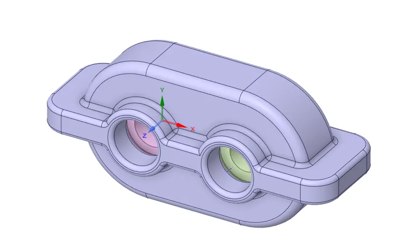
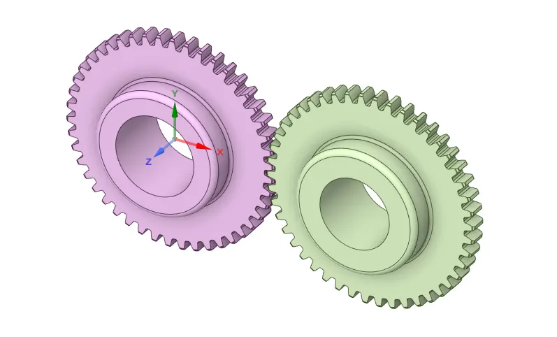
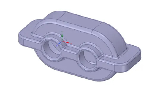
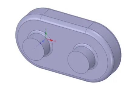
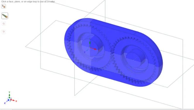
The picture below shows a 3D view of a gear box. If you hide the housing, you will have a better opportunity to see the left gear and the right gear. The image that can be seen below is a 3D representation of gears.

• First things first: let's get the fluid volume out of the way. For that, follow these steps:
• preparation -> volume extract -> pick the fluid volume by selecting all the borders of 4 holes -> Then press the ok button.
• The tree will then receive a new object at that point.
• Then hide the volume of the solid, and what's left is the volume of the fluid that we made.
• Now that we have reached this point, we need to cut this body in half so that we may extract the 2D geometry from the centre plane.
• To begin, create planes by first picking plane in design and clicking on origin. This will result in the creation of two planes with X, Y, and Z planes.
• We use the split body command in spaceclaim, which is now in the process of being developed. This command allows us to split the geometry into two parts by selecting the geometry and the plane and then deleting the other part.
• The transverse image of the interior is now visible to us.
• If you now choose the top portion of the remaining geometry, you will be able to view the yellow top face component, which is exactly what we want.
• In order to extract that region, we need to choose that face, copy it, then open a new design, paste it, and save it. Only then will we be able to extract that area.
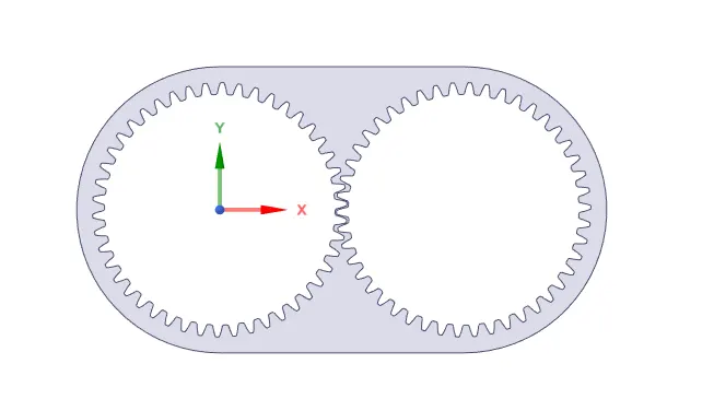
• Now you should reset the configuration, import the 2D geometry that was saved, and then launch the meshing module.
• The final 2D geometry that we replicate can be seen in the image that follows.

Meshing –

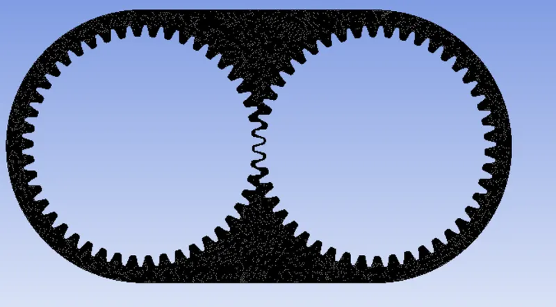
• It is recommended to utilise a tetrahedral mesh rather than a hexahedral mesh for the fluid domain since the fluid domain is made up of multiple curves rather than straight-line geometries (which may lead to inaccurate results).
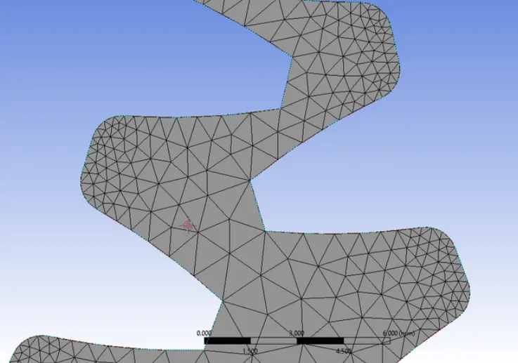
• As a result, a method known as "All triangles" was used to analyse the 2D fluid domain.
• The size of the element remained maintained throughout the process at 0.8mm.
• In addition to this, the option to "Capture proximity" was activated, and the number of cells that should be skipped over gaps was set to 1.
• Because of this, we are able to record microscopic gaps within the geometry, which contributes to the mesh's increased precision.
• After that, the mesh was constructed, and the total number of cells in it was 15,918.

Problem Setup :

• In order to prepare for our problem, we launch Fluent and configure the initial conditions, boundary conditions, material, and so on.
• First things first, we do a quality check on the mesh by using the perform mesh check under domain command.
• If there is no indication of an error in the console window, then we are free to move on.
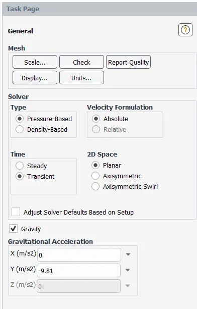
• Then we move on to setting up physics, where we pick the solver, viscous model, etc.
• In order to solve our model, we make use of a transient state pressure-based solver.

Physics :

General :

Solver type : pressure based

time : transient state

velocity formulation : absolute

• In order to make use of gravity, we need to set the value of Y to -9.8 m/s2; this is because gravity pulls in the opposite direction of Y.

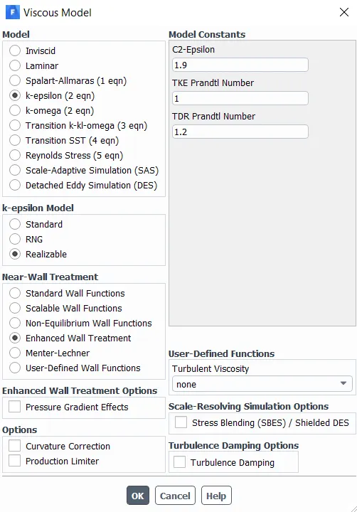
models :

viscous model : K-epsilon realizable model with enhanced wall treatment.

Material : Fluid -1 : Air

Fluid -2: Engine oil (density - 880 kg/m^3 , Viscosity - 0.121 kg/ms )

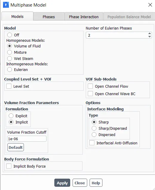
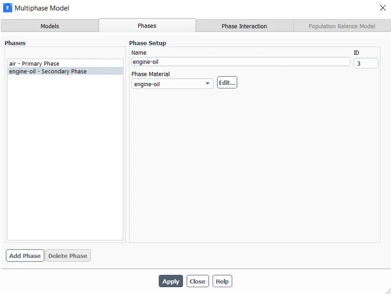
• And in the phases option, given that we choose two stages and gave them names before choosing phase,
• Change the name of the primary phase to air, and make air the material of the primary phase.
• For the secondary phase, the name should be changed to water, and the phase material should be changed to motor oil.
• Then, in order to perform patching, we must initially initialise, and after that, we perform hybrid initialization.
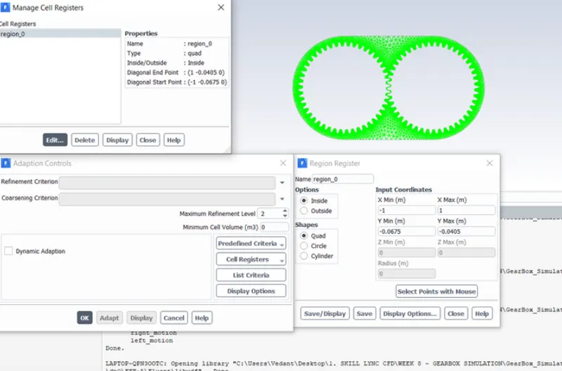
• However, before we can begin initialization, we need to identify or define a zone of cells where the fluid must be, such as 20% of immersion, in order to get the 20% of the height that we notice from the spaceclaim. When designing the dynamic mesh, we also make a note of the location of the centre of gravity for use in the process. WE mark by making use of the adapt/mark command and then creating a region by giving the values that produce the appropriate region.
• In the patch, pick engine oil for the phase, and under variables, you should now be able to see the volume fraction.
• Now, patch the value fraction value of 0 to another domain, and patch the value 1 to the region that we have just constructed, which can be found in the registers to be patched.
• Now that we are almost ready to start the simulation, we need to generate a contour for the volume portion of water. This is done so that we can validate the patching.
• Now that the patching has been completed, we can test it by generating a contour of the volume proportion of engine oil.
• Go to the solutions tab, then graphics, then contour, and then follow the instructions there. in the contour of menu, choose phases; then, under that, choose volume fraction; then, for phase, choose engine oil; finally, choose full domain; and last, click the save and show button.
• Then you will be able to see the initial values for the volume fraction of engine oil across the complete domain, where you will notice that in the lower zone it is set to 1, while in the upper region it is set to 0.
• As a result, we are able to draw the conclusion that our initialization was done correctly.
• After that, we will need to configure the dynamic mesh.
• In order to do so, we need to load the UDF, choose, under the user defined menu item, then pick the function menu item, then select the compiled menu item, then add and utilise the built in compiler to construct the UDF, and then load it.

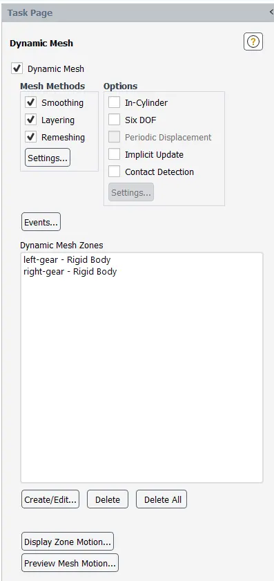
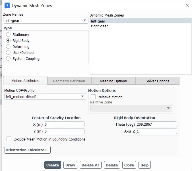
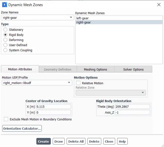
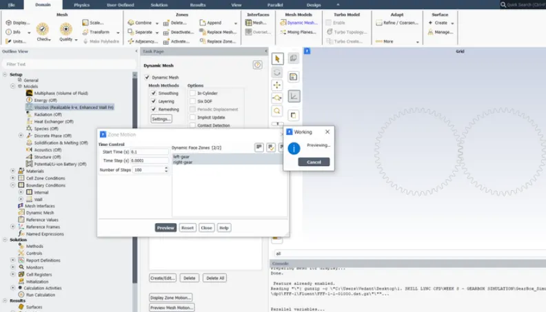
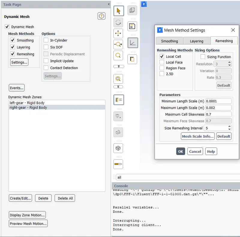
• Now, within the mesh module, choose dynamic mesh, and then within that, choose smoothing, layering, and remeshing. After that, we will need to construct dynamic mesh zones.
  Chose "create" from the drop-down menu under "dynamic mesh zones," and we need to construct,
  For left gear: -> select for type - rigid body -> for motion UDF/profile - select left motion -> and for centre of gravity - give value as (0,0,0), which is the centre of gravity we noted: -> For right gear: -> select for type - flexible body -> for motion UDF/profile - select right motion -> and for right gear: -> select for type - After that, select the Create option.
• In the same way, generate the right motion by providing, for the motion UDF/profile, we select the right motion, and for the centre of gravity, we provide the value (0.115,0)m.
• After that, you will notice that two zones have been established in the dynamic zones: the left gear zone and the right gear zone.
• By selecting pick display zone motion as well as setting time control and preview, you will be able to watch the motion of the gears.
• You will notice that the gears are turning.
• As a result, we are able to draw the conclusion that the UDF was correctly set up.
• The next step is to perform the initialization and patching steps once more. In addition to this, we need to develop an animation so that we can observe how the solution or the volume fraction of water varies as the problem is solved.
• steps: Activities -> solution animation -> preview -> set the appropriate view and utilise active -> and label it as volume fraction of water animation.
• Then, in the method of solution for the pressure velocity coupling, the SIMPLE scheme is utilised. PRESTO is chosen to calculate the pressure, whereas the second order upwind technique is employed to calculate the momentum. The first order implicit scheme has been used for the transient formulation because it yields superior results and also ensures the stability and convergence of the residuals.

Solving:

• After that, we are prepared to solve.
• We perform the simulation by specifying that the number of time steps should be set to 1000 and the time step size should be 1e-4.
• In this part of the UDF, the angular velocity is written as 200 rad per second. It indicates that omega equals 2 pi times N divided by 60, therefore N equals 1909.8593 rpm, which is equal to 31.8309 revolutions per second.
• Therefore, the time required for one spin is 1/31.8309 seconds, which is equal to 0.031416 seconds.
• In this case, we conducted the simulation for a total of 1000 time steps with a time step size of 0.0001. Since the entire time was 0.1 seconds, this indicates that we ran for more than three rotations, which is sufficient for our investigation.

Post processing:

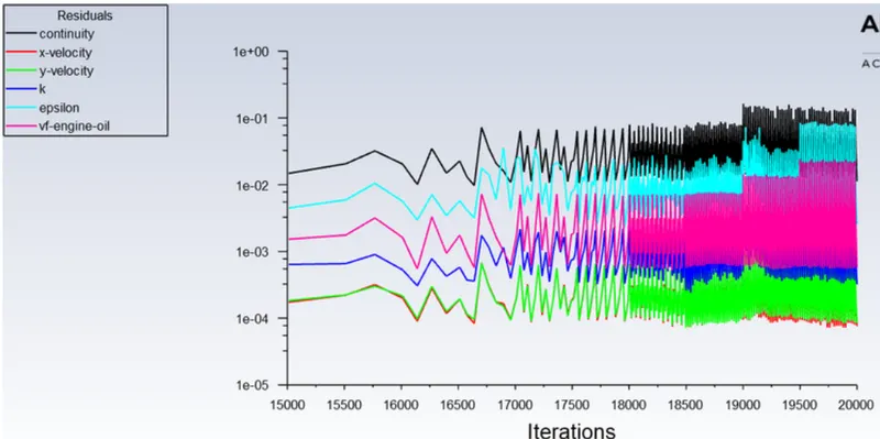
• As can be seen in the plot below, the residuals have reached a point of convergence.
• 

Animation:

• An animation showing the effect of fluid sloshing around inside a gearbox, with 20% of the gears being immersed in the fluid (engine oil).
• https://youtu.be/izjb5FaPJek

Case -2 :- 30% of immersion with fluid - Engine oil :

• In terms of the geometry and the mesh, everything is the same as it was in the previous situation.
• Coming to set up, the only difference that has occurred is that the immersion level is now 30%.
• Therefore, we provide a variety of values for the coordinates that are used for marking. For example, the values that we provide here are 30% of the height measured from the base.
• The fluid in question is also the same in this instance.
• Everything else is exactly the same as in the previous situation.
• After that, we let the simulation run for 0.1 seconds, during which time it will take 1000 time steps with a time step size of 0.0001.
• Therefore, let us immediately begin the simulation, and after it is finished, we will process the data.

Post processing :

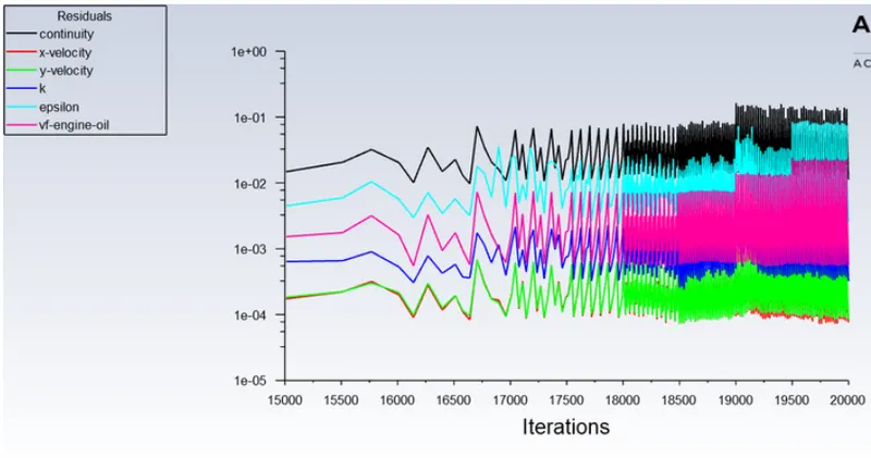
• As can be seen in the plot below, the residuals have reached a point of convergence.
• 

Animation :

• An animation showing the effect of fluid sloshing around inside a gearbox, with 30% of the gears being immersed in the fluid (engine oil).
• https://youtu.be/_KRrpt7MvSc

Case -3 :- 20% of immersion, fluid - n-heptane (c7h16) :

• In terms of geometry and mesh, everything is the same as it was in the two situations before this one.
• Coming to the setup, the only difference is that from here on out, the immersion will be at 20%.
• Therefore, we provide a variety of values for the coordinates that are being marked; for example, here we provide coordinates for values that are 20% of the height from the base.
• In this scenario, the fluid in question is n-heptane, which has the formula C7H16.
• Everything else is exactly the same as in the previous examples.
• After that, we let the simulation run for 0.1 seconds, during which time it will take 1000 time steps with a time step size of 0.0001.
• Therefore, let us immediately begin the simulation, and after it is finished, we will process the data.

Post processing :

• You can observe from the below plot the residuals has converged.
• 

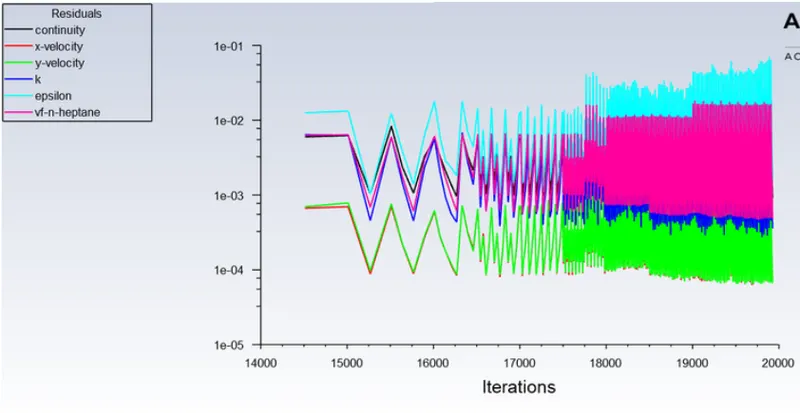
Animation :

• Effect of fluid sloshing around inside a gearbox, animated. N-heptane fluid is immersed to a depth of 20%. (c7h16).
• https://youtu.be/3lPRUDDDLto

Case -4 :- 30% of immersion, fluid - n-heptane (c7h16) :

• In terms of geometry and mesh, everything is the same as it was in the three situations that came before this one.
• Coming to the setup, the only difference is that from here on out, the immersion will be at 30%.
• Therefore, we provide a variety of values for the coordinates that are used for marking. For example, the values that we provide here are 30% of the height measured from the base.
• In this scenario, the fluid in question is n-heptane, which has the formula C7H16.
• Everything else is exactly the same as in the previous examples.
• After that, we let the simulation run for 0.1 seconds, during which time it will take 1000 time steps with a time step size of 0.0001.
• Therefore, let us immediately begin the simulation, and after it is finished, we will process the data.

Post processing :

• You can observe from the below plot the residuals has converged.
• 

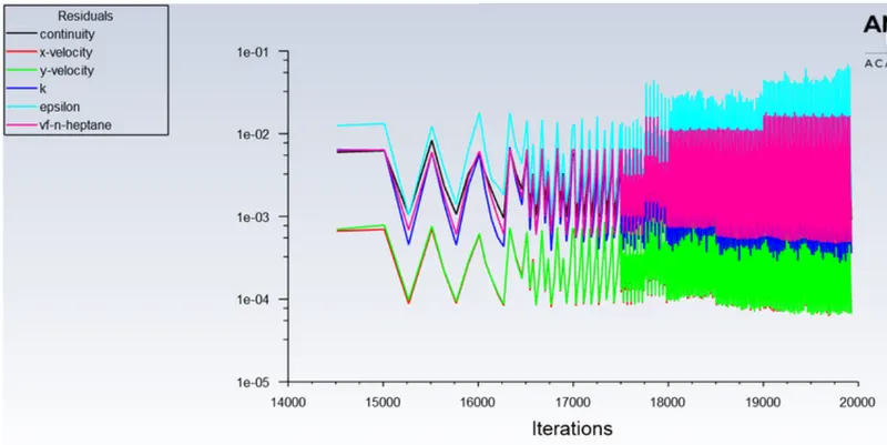
Animation :

• Effect of fluid sloshing around inside a gearbox, animated. N-heptane fluid is immersed to a depth of 30%. (c7h16).
• https://youtu.be/Ou6pmwa6Tyc

Conclusions:

• Let's wrap up by contrasting the outcomes across the board and talking about the most common mistakes that will crop up during the simulation. An error that reads "Dynamic mesh failed." and 'Negative cell volume detected' error.
• If you watch the animations closely, you'll notice that fluid flows upwards from the bottom of the gear box and then returns through the sides of the gear box after meeting at the top.
• When you inspect the gears, you'll see that the fluid is effectively reaching each and every one of the teeth.
• However, in examples 2 and 4, where the immersion is 30%, there is still fluid in the sump after the first rotation has finished, allowing for greater lubrication. This is in contrast to cases 1 and 3, where all of the fluid has been used for the first rotation, leaving the second rotation's sump nearly empty and requiring longer time for the top fluid to backtrack downhill to the sump.
• Therefore, the lubrication is improved when there is a greater degree of immersion.
• Because engine oil has a higher viscosity than n-heptane, it adheres very strongly to the gears and lubricates them more effectively, as can be seen in the animations, as compared to the other fluids used (i.e., cases 1, 2, and 3, 4). This can be seen by comparing the fluids used in cases 1, 2, and 4.
• In scenario 2, the gears are immersed in fluid engine oil to a depth of thirty percent, making them exceptionally well lubricated. This is the best situation out of all the possible ones.

Common errors that will occur in the simulation :

Dynamic mesh failed error :

• This problem manifests itself whenever an attempt is made to update the dynamic mesh but is unsuccessful.
• It could be due to a variety of factors, such as a negative cell volume, for example.

Negative cell volume detected' error :

• If the mesh is getting too compressed/deformed or skewed in a dynamic simulation, which causes the mesh quality to deteriorate even to a point where cells turn into negative cell volume when the mesh moves too far at a given time step, it leads to negative cells, negative cell volumes are usually produced. This happens when the mesh is getting too compressed/deformed or skewed. When the mesh has been modified in such a way as to result in a negative cell volume, the negative cell volume error will be displayed (non-physical).
• This issue could have been caused by a number of different circumstances, including, but not limited to:

(1) overlapping nodes; and

(2) considerable mesh motion (relative to cell size) every step.

• These elements are connected in some way.
• This occurs as fluent do not have enough time to remesh.
• In order to prevent the mesh quality from deteriorating to such an extent, one possible option is to remesh the area at more frequent intervals.
• If you want to prevent significant mesh displacements, try decreasing the time step. In order to prevent the severe deformation of boundary layers or near-wall mesh cells, another possible option is to raise the stiffness of the mesh in the area immediately adjacent to any solid walls that are present in the simulation.