Week 7 - CHT Analysis on a Graphics card

AIM:

To perform a steady-state conjugate heat transfer analysis on a motherboard and to understand how the heat transfer takes place from the energy source defined in the simulation.

THEORY:

CHT ANALYSIS:

Conjugate Heat Transfer (CHT) is a type of heat transfer analysis between both solids and fluids. CHT involves both convection (Between fluids) and conduction (between solids) heat transfer, as well as both forced and natural convection. So in CHT analysis, we have to consider both the convection in the fluid medium and the conduction in the solid medium to analyze how the heat transfer happens. This will provide the data in that medium which we can be able to vary in accordance with its application.

FLUID & SOLID INTERACTIONS:

The temperature field and the heat flux are continuous at the fluid/solid interface. But the temperature field can rapidly vary in a fluid in motion which is close to the solid and the fluid temperature is close to the solid temperature. In far from the interface the fluid temperature is close to the inlet fluid temperature. The distance where the fluid temperature varies from the solid temperature to the fluid bulk temperature is called the thermal boundary layer.

CHT APPLICATIONS:

• To analyze the effective heat transfer in the heat exchanger
• To analyze the effectiveness of heat transfer in the electrical and electronic components for forced and natural convection.
• To understand the radiative heat transfer in the components where the fluid medium is mainly air.

INTRODUCTION:

Now we are going to analyze the given model based on the following cases.

CASE I : Automatic mesh (Base line set up with the flow of 1m/s)

CASE II : Meshing refinement is done for every part in the board with a flow of 1m/s. Have to analyze how the meshing refinement produces the results.

CASE III : With the refined mesh have to increase the flow to 3m/s and observe the temperature effects on the board.

CASE IV : With the same refined mesh have to increase the flow to 5m/s and observe the temperature effects.

PROCEDURE:

GEOMETRY STUDY:

To perform the simulation we have to understand how the model works, how the physical attributes has an effect on the model, what parameters to be consider for simulation and how to define the energy source. By the clear view of study we can get an idea of how to proceed further with the simulation.

We are having the model of Motherboard, which is a key part of the functioning of a PC. It consists of RAM, ROM, Processor, and some electronic components which supports the entire power circuit required for the components. The model provided a typical representation of the motherboard, not the exact one as we are initializing our project in CHT. So the major components we consider here for running a simulation in our model is of

• Base
• Fins
• Processor

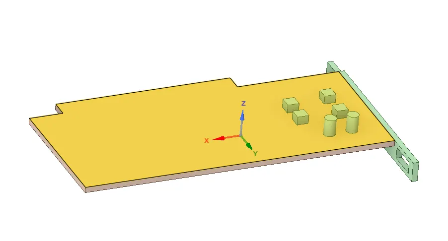
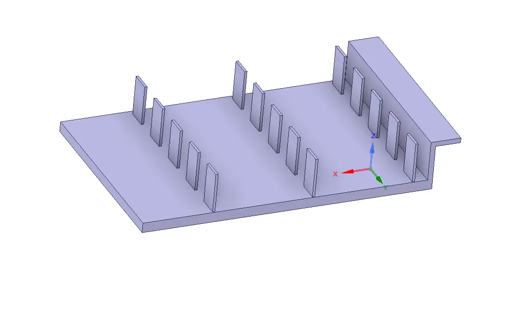
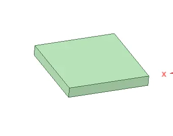
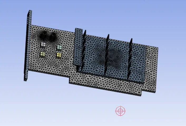
Initially we open the model in space claim to share the topology for the individual parts. By sharing the topology we can avoid the Non-conformal mesh. The non-conformal mesh will not give us a better results. This is because each part do have a different shape and size, depending upon the mesh size also varies. If the part is assembled, the mesh will not overlay with each another and forms a non-conformal mesh. To avoid these we have the use SHARE PREP option to create the conformal mesh between the parts.

MESHING:

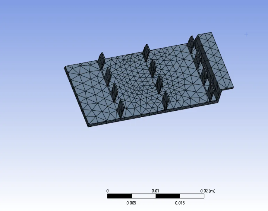
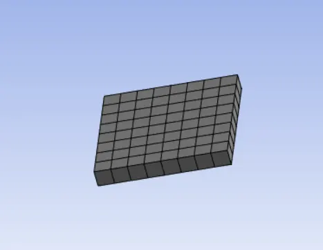
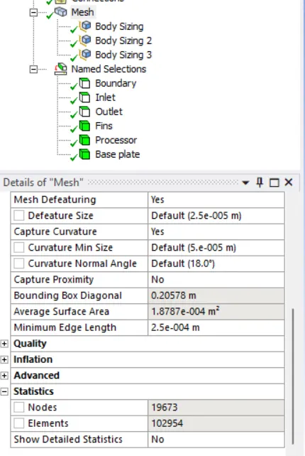
CASE I: (Number of Elements - 102954)

Geometry is imported in the meshing interface and automatic meshing is done and by providing body sizing provided the coarse mesh.

Base Plate - 3mm

Processor - 1mm

Fins - 2mm

Enclosure - 5mm

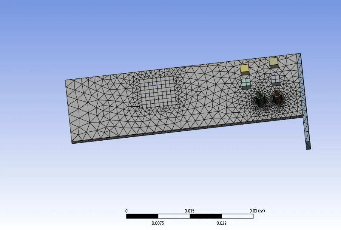
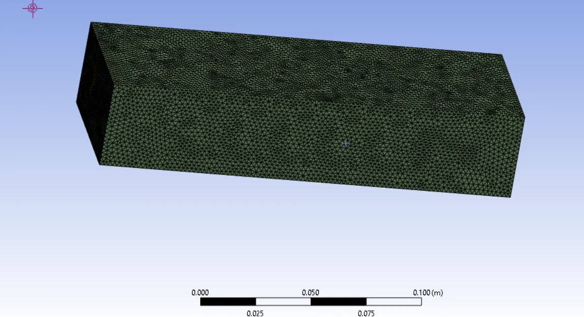
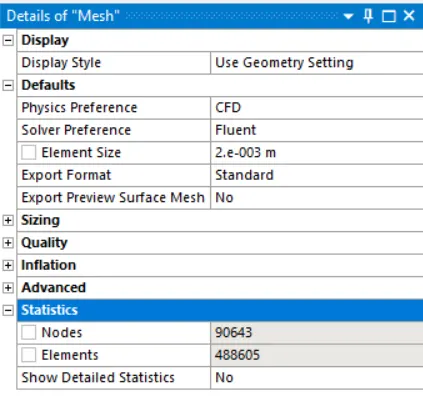
CASE II, III, & IV: (Number of elements - 488605)

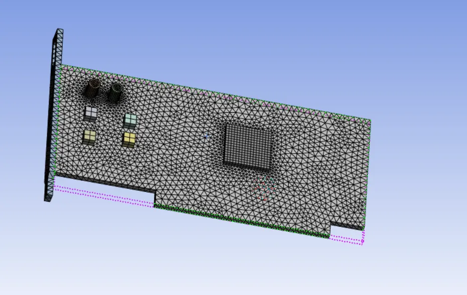
Meshing refinement is done by providing various element lengths for each part in the processor.

Base plate - 0.5mm

Processor - 0.3mm

Fins - 0.5mm

Enclosure - 2mm

METHOD SELECTION:

Turbulence Model : K- Omega SST Model

Solver : Pressure Based Solver

Time : Steady

Method : Coupled

Temperature : 300k

Velocity : Case I - 1 m/s

Case II - 1 m/s

Case III - 3 m/s

Case IV - 5 m/s

MATERIAL SELECTION:

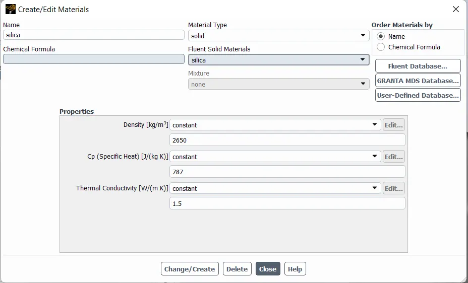
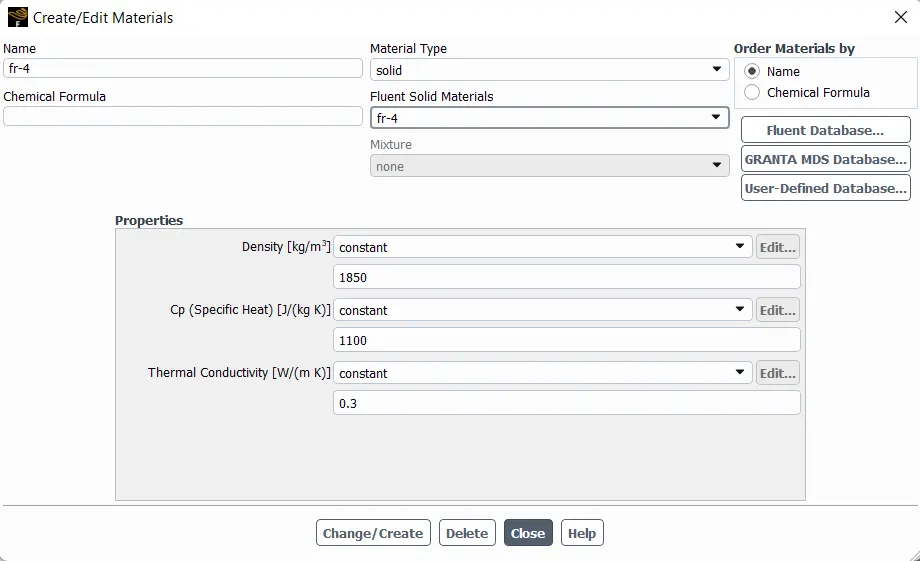
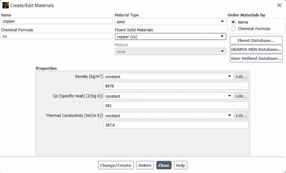
For the model we have, there are three major components we considered. Each component do have different types of material according to thier purpose of use. So we have to choose the correct material properties depending upon the component nature. And we have to properly choose whether the component is of solid or fluid.

Processor: (Silica is considered)

Base Plate: (FR4 material is considered)

Fins: (Copper is considered)

ENERGY SOURCE:

Here in motherboards, we are having multiple tiny electronic circuits which will produce heat during its operation. But one of the major source of heat producing component is of Processor. Processor are the major part where all the functions are done inorder to run the operation, so it will raise it to the high temperature. So we can considered this as our energy source. And we have to analyze how to taken away the heat from the processor for effective running of PC. For that we have to provide the input of energy value to the source.

We considered that the average power required for doing the minimal operation as 65W, whereas normal processor would take two times more than provided power during high usage time. By considering all the power used will be converted as a thermal energy, thus by we can calculate the energy density by a simple formula.

`S = (65W)/(64mm^3)`

By converting all the values we got, S = 1015625000W/m3

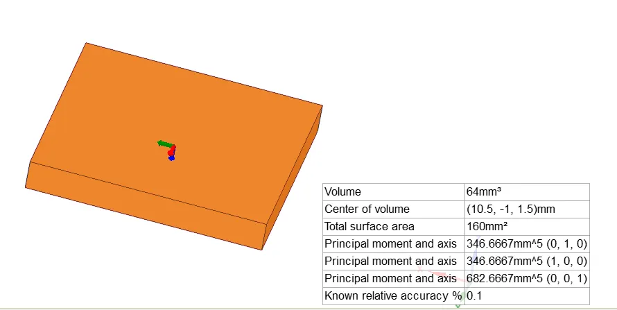
While selecting the materials for the processor, we have to provide the value of energy term as a constant through out the simulation.

PLOTS:

RESIDUALS:

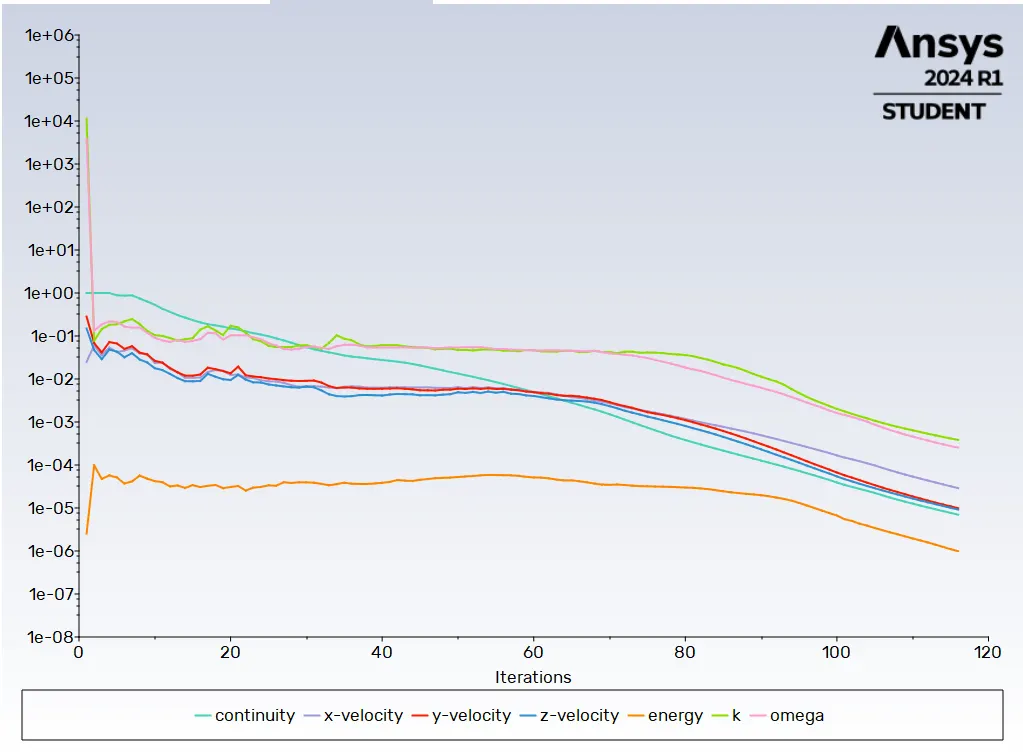
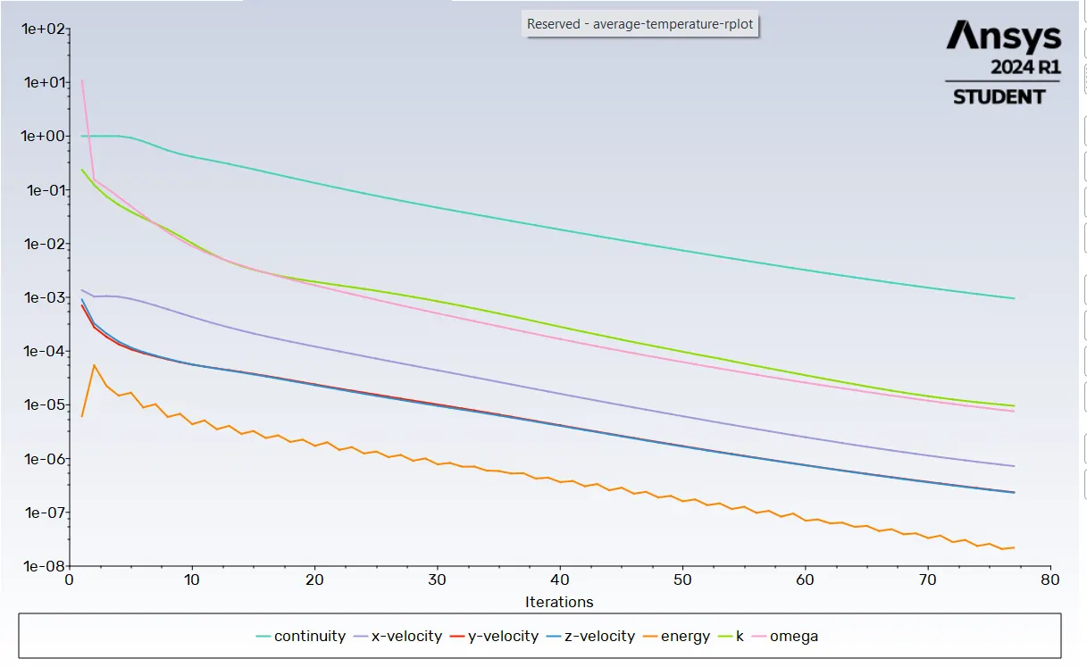
CASE I:

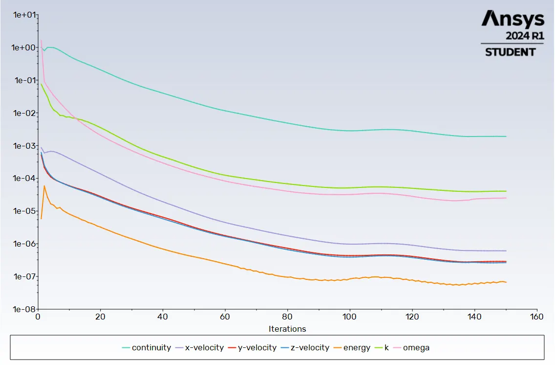
CASE II:

CASE III:

CASE IV:

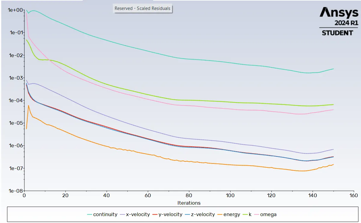
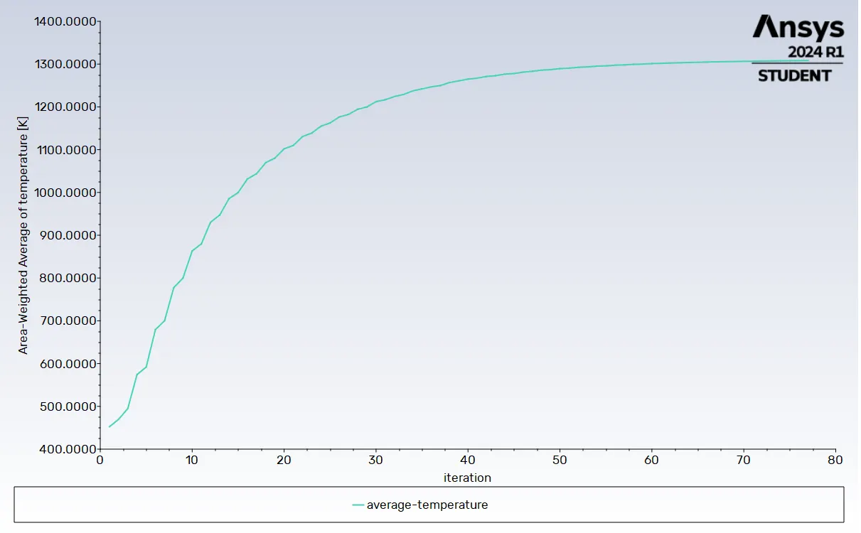
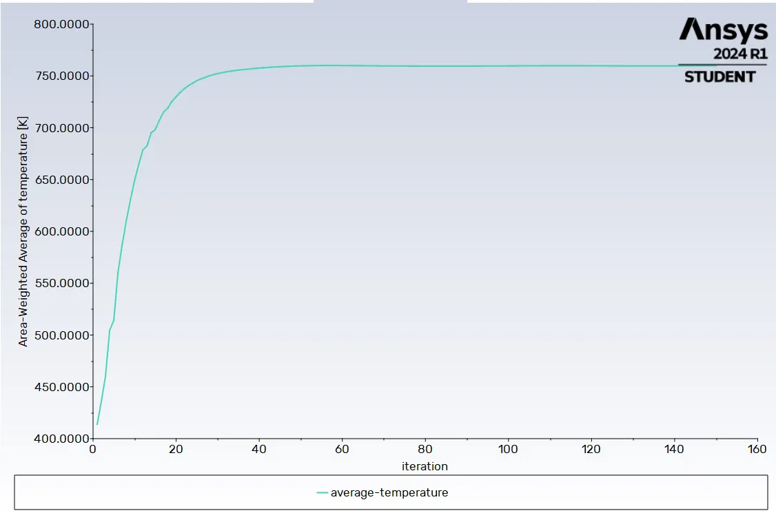
We can able to tell the solution is converged or not depending on the graph during our simulation. For cases I and II, the solution converged during the simulation process itself by throwing the converged message. But for our case III and IV, it is not like that, so we have to decide whether we run the simulation to further steps or not.

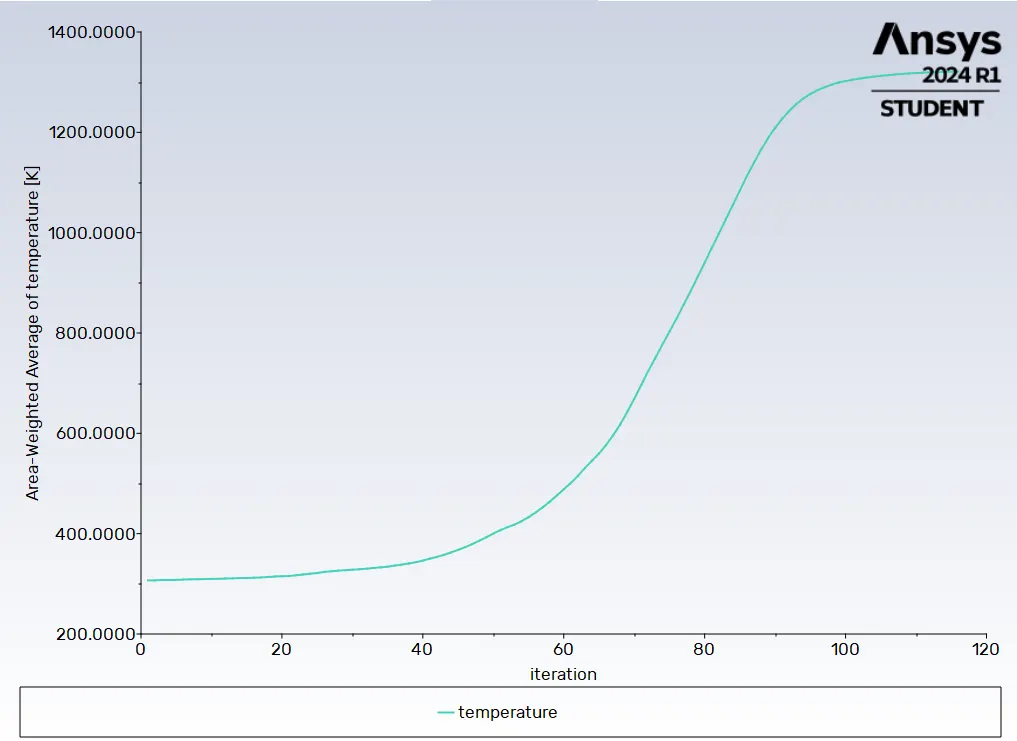
We can tell by looking at the residuals graph or our end result graph. Here we are expected to find out the average temperature graph. So if the graph values do not deviate much and give the atmost same results for each and every iteration, then we can conclude that the solution is converged. The same for the residuals as well, if the results follow the linear same path then we can be able to decide whether the solution is converged or not.

AVERAGE TEMPERATURE:

CASE I: (1321K)

CASE II: (1308K)

CASE III: (760K)

CASE IV: (616K)

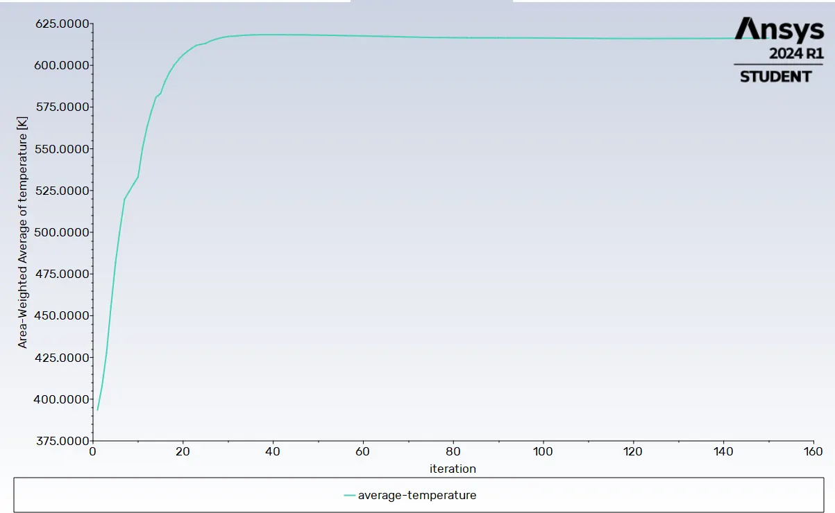
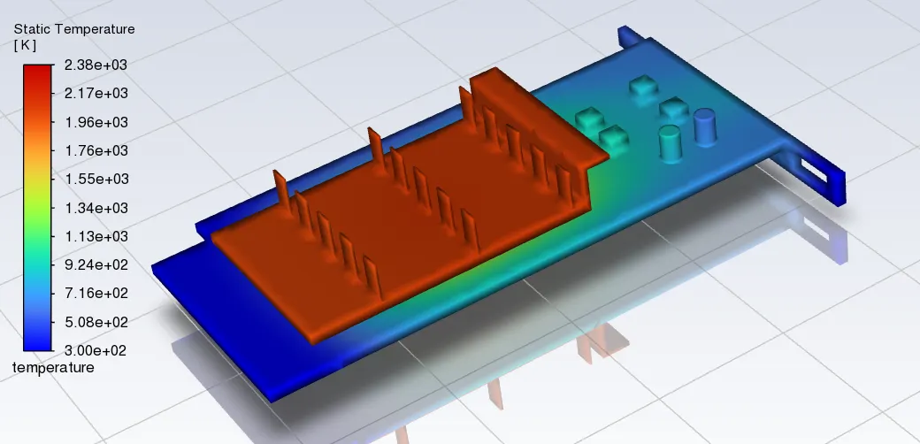
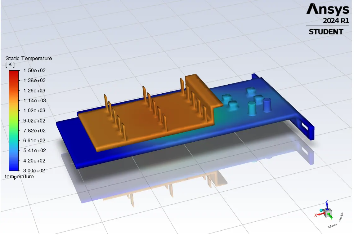
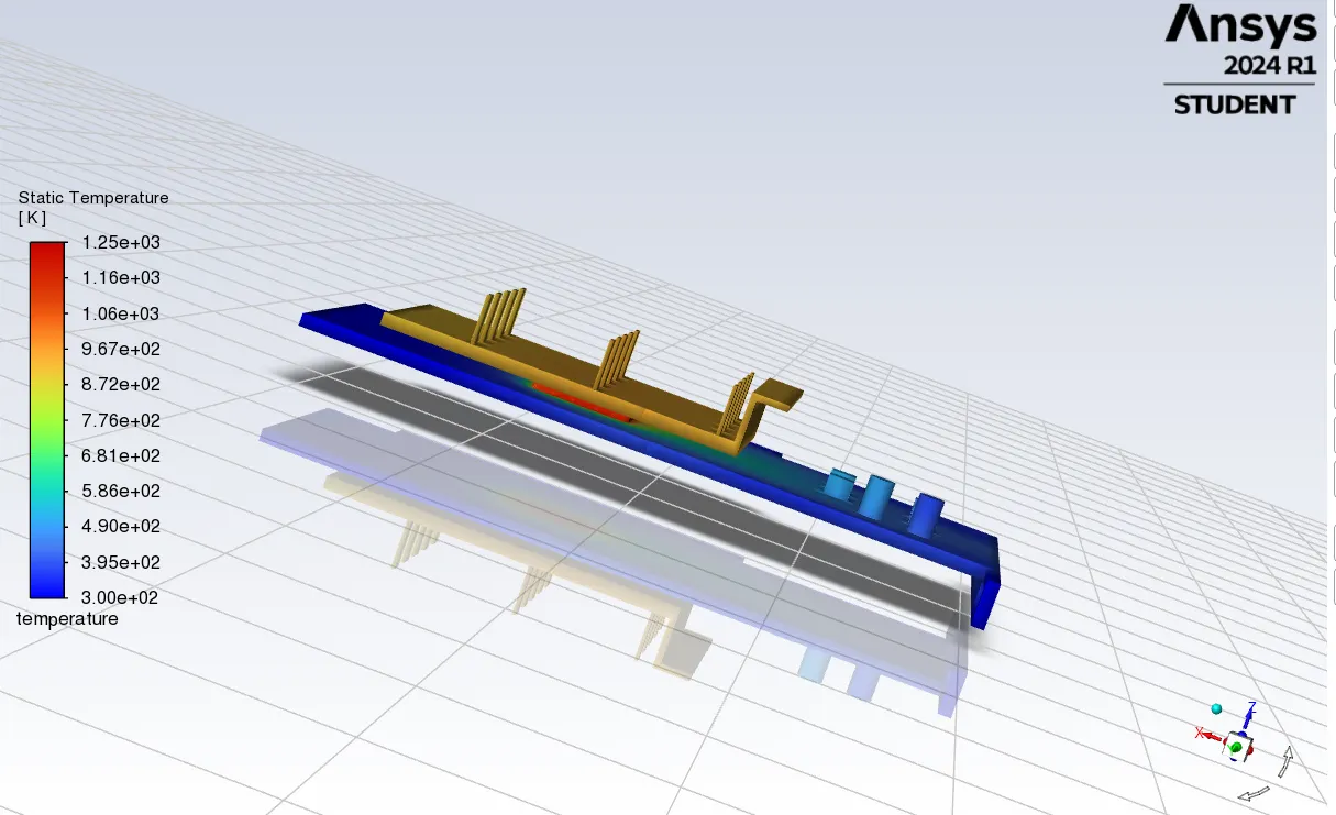
By looking at the temperature graph, clearly indicates the accuracy of the results. When we are increasing the velocity of input from 1m/s to 3m/s and to 5 m/s, the average temperature gradually comes down. This is all because of the convection of heat between the fins to the air. When we increase the flow velocity of air, the air that passes through the fins will increase, that transfer high amount of heat to the air. This leads to the average temperature being reduced compared to that of with lower velocity.

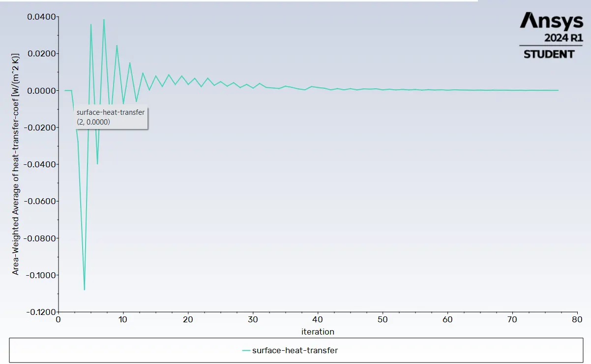
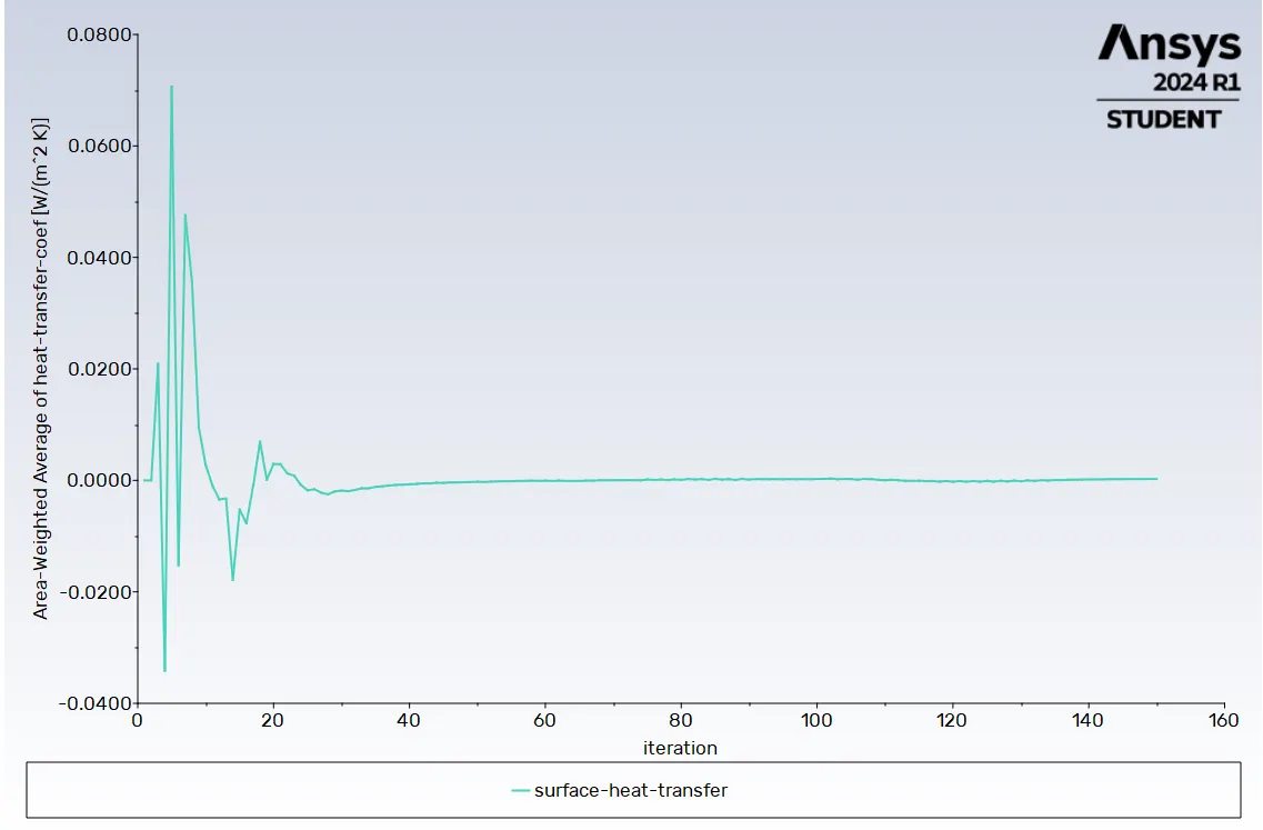
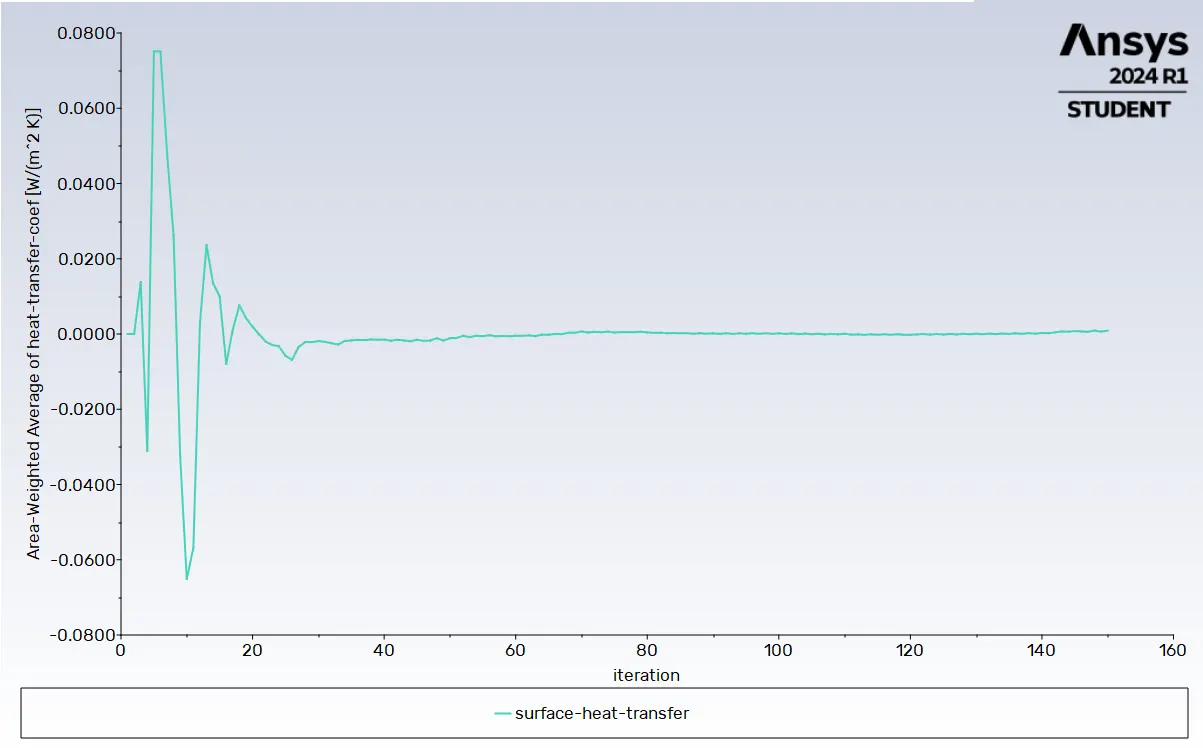
SURFACE HEAT TRANSFER:

CASE I: (0.00102436 W/m2 K)

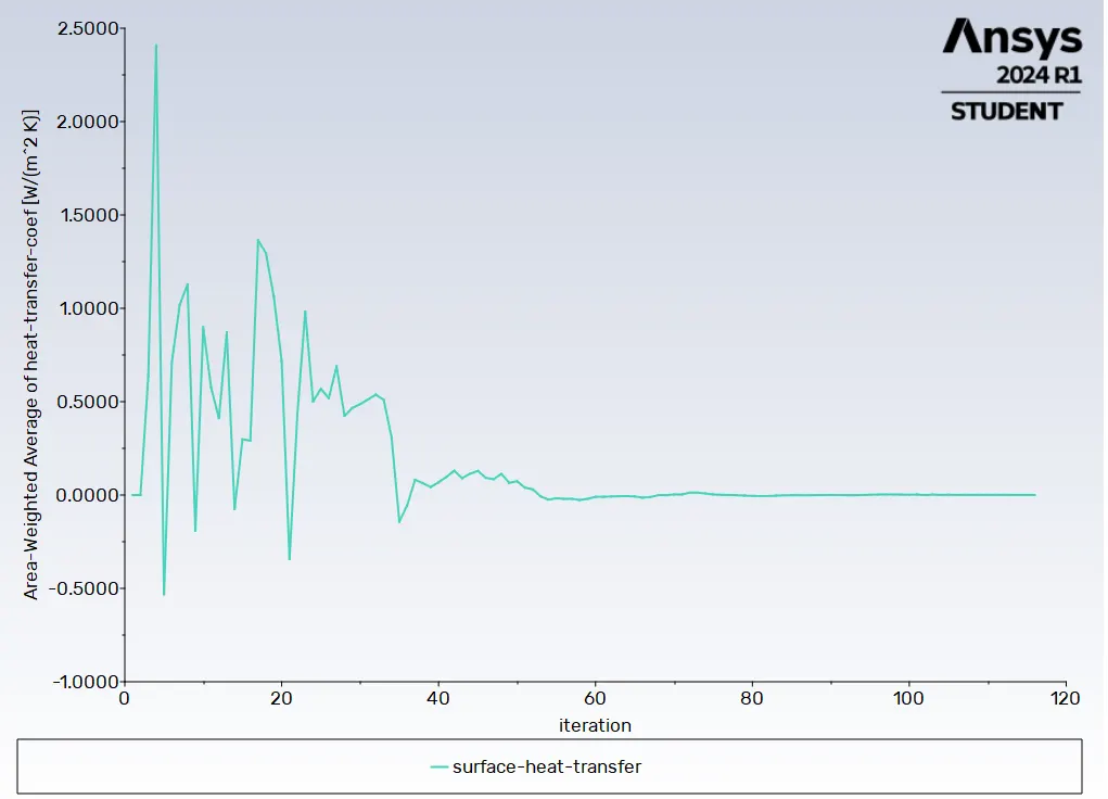
CASE II: (0.0001576 W/m2 K)

CASE III: (0.0002279 W/m2 K)

CASE IV: (0.0009007 W/m2 K)

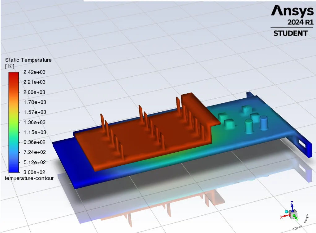
TEMPERATURE CONTOUR:

CASE I:

CASE II:

CASE III:

CASE IV:

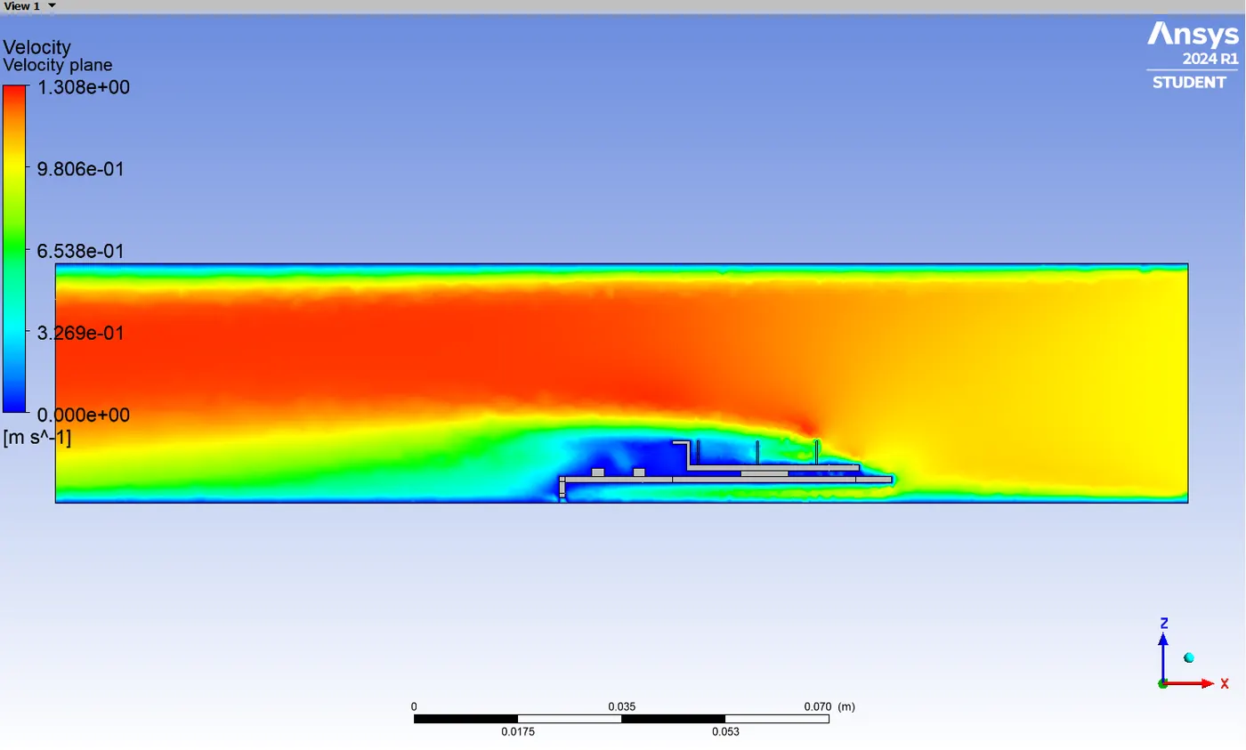
VELOCITY CONTOUR:

CASE II:

TEMPERATURE CONTOUR:

CASE II:

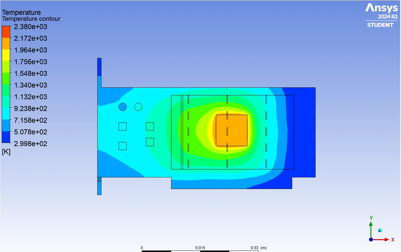
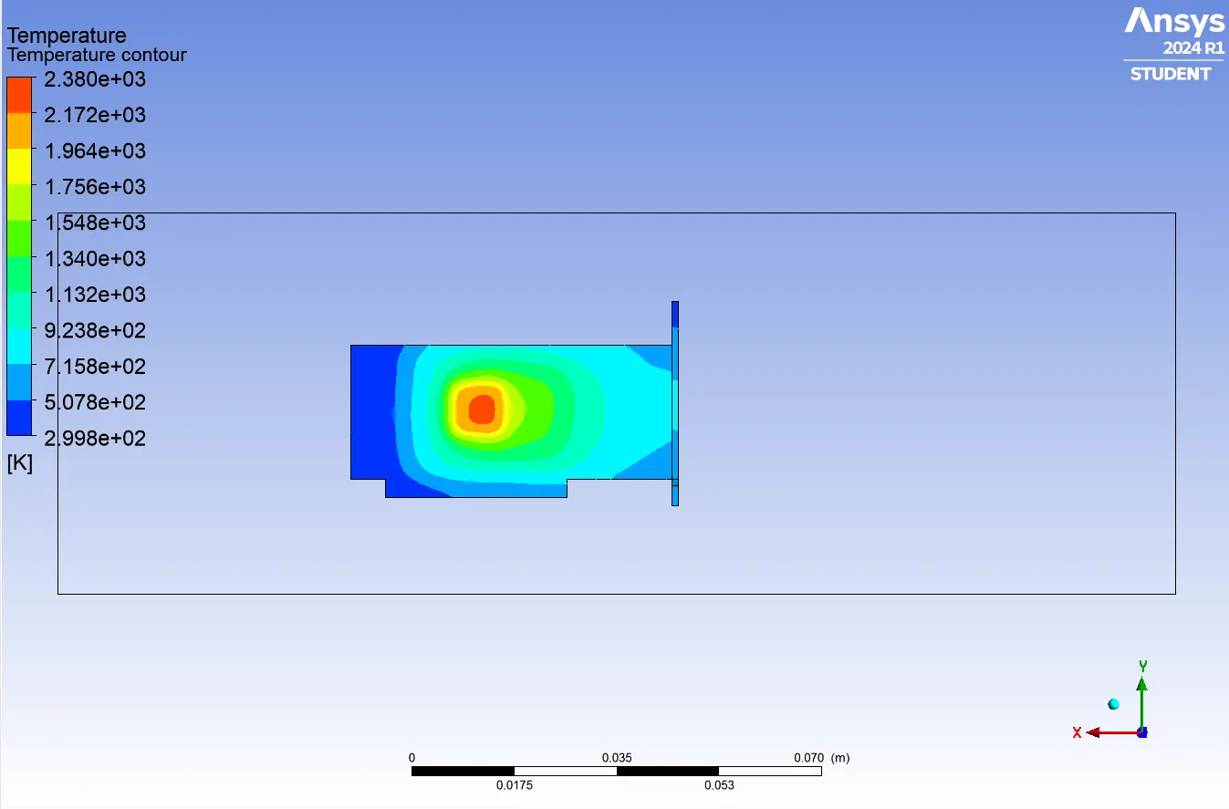
OBSERVATIONS:

S.No	Velocity (m/s)	Number of Elements	Maximum temperature	Average temperature (K)	Surface heat transfer coefficient (W/m2 K)
CASE 1	1	102954	2420	1321	0.00102436
CASE 2	1	488605	2380	1308	0.0001576
CASE 3	3	488605	1504	760	0.0002279
CASE 4	5	488605	1253	616	0.0009007

RESULTS:

Thus we simulate the Conjugate Heat Transfer analysis on a given model of motherboard and we observe the changes of its temperature according to the variation in velocity profile. And we understand about the hotpoints in the model when we are performing the analysis for variation of flow.

OUTCOMES:

• Understanding of variation of temperature according to velocity profile.
• Identifying the solution convergence by looking out at the graph.
• Importance of identifying the hotspot in the model and understanding about its effects during the design phase.
• Clear outview of Conjugate Heat Transfer theory.