Week 3 - Solving second order ODEs

AIM:

To plot the Displacement and Velocity curve for the motion of a simple pendulum. And to stimulate the motion of the simple pendulum using animation.

PROCEDURE:

PROGRAM 1 - For Plotting the Displacement and velocity curve with respect to time given.

clear all
close all
clc

%Input Variables to be given
b = 0.05; %Damping coefficient
l = 1; %length of the string in m
m = 1; %Mass of the bob suspended in kg
g = 9.81; %Acceleration due to gravity in m/s^2

%Initial Conditions
theta_t = [0;3];

%Time given
t_span = linspace(0,20,200);

%Function used for pendulum motion
[t, results] = ode45(@(t,theta) Ode_SP_Function(t,theta,b,l,m,g),t_span,theta_t);

%Plotting of Displacement and Velocity curve
figure(1)
plot(t,results(:,1),'LineWidth',1.5) %New command used I
hold on
plot(t,results(:,2),'LineWidth',1.5) %New command used II
grid on
xlabel('Time in Seconds')
ylabel('Velocity and Displacement Curve')
title('SIMPLE PENDULUM','color','m','fontsize',15)
axis([0 20 -7 7])
legend('Displacement of Bob','Velocity')

%Plotting of Animation for Simple Pendulum
figure(2)
displacement = results(:,1);
velocity = results(:,2);
ct=1;

for i = 1:length(displacement)
    x0 = 1.5;
    y0 = 1.5;

    x1 = 1.5-(l*sin(displacement(i))); %Formula for taking the position of pendulum in X
    y1 = 1.5-(l*cos(displacement(i))); %Formula for taking the position of pendulum in Y

    
    grid on
    plot([0.5 2.5],[1.5 1.5],'linewidth',5,'color','r')
    hold on
    plot([x0 x1],[y0 y1],'linewidth',2,'Color','k')
    plot(x1,y1,'o','markersize',20,'markerfacecolor','r')
    axis([0 3 0 1.5])
    hold off
    title('Animation of Simple Pendulum','color','m','fontsize',15)
    M(ct) = getframe(gcf);
    ct=ct+1;
   

end

movie(M);
videofile = VideoWriter('Animation of Simple Pendulum.avi','uncompressed AVI');
open(videofile)
writeVideo(videofile,M)
close(videofile)

CODE EXPLANATION:

• In the start, I provided the input variables that is provided in the question. And also I provide the initial condition of Angular displacement and angular velocity in terms of matrix. Then I provided the interval of time using the linspace command.
• Then, I called the function already created in the another program. Here I use ODE45 command to solve the Differential Equation. The results of the function is stored in a matrix format names as [t,results], where t is the time interval and results has two column and 200 rows. Out of these First row is for Displacement and Second row is for Velocity.
• Here I learned one new command. That is calling of one row in two row matrix using : command. For plotting the displacement curve, I choose first row from results by providing (:,1) and for plotting the velocity curve , I choose the second row from the results by providing (:,2).
• After that, I label the axis name using xlabel() and ylabel() command and given the title of the plot.
• And I align the axis by providing required axis numbers. Then I also provide the legend.
• Then for plotting the animation of the simple pendulum, I seperate the results matrix by providing them with the name. The first row is named as displacement and the second row is named as velocity.
• Then I use the for loop command for the variable displacement. This is due to we want the stimulation of the simple pendulum. I used the simple trignometry formula for calculating the position of Bob in X and Y.
• After that, I plot the Horizontal line considering it as the wall where pendulum suspended. And then I plot the length of the string and at the end of the string I plot bob with the marker command.
• Then using the command getframe(gcf), I get each and every frame obtained in for loop. Because for every loop finalization I give ct=ct+1; It will increment the loop count upto the all value is calculated in displacement row.
• Then using VideoWriter command I saved it as a video. And open() command is used to open the video at the end of stimulation. And writeVideo() write the video file in Movie M. And close() command is used to close the video after the video is played.

PLOT:

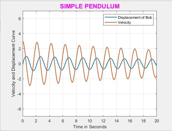
This is the plot obtained from Displacement and velocity curve.

PROGRAM 2: Function used for the simple pendulum

%Function to calculate Displacement and velocity curve for simple pendulum
function [dtheta_dt] = Ode_SP_Function(t,theta,b,l,m,g) %function format
theta1 = theta(1);
theta2 = theta(2);
dtheta1_dt = theta2; %Formula used obtained by converting second order ODE into two First order ODE
dtheta2_dt =-(b/m)*theta2-(g/l)*sin(theta1); %Formula used obtained by converting second order ODE into two First order ODE
dtheta_dt = [dtheta1_dt ; dtheta2_dt]; % Values stored in matrix form for input

end

FUNCTION EXPLANATION:

• First line is the Function format, where we have to given the variables required for calculating the function.
• In second and third line, we indicates the theta value. This is for at the end of the function we given the name of theta value in a matrix form.
• In fourth and fifth line, we have the second order ODE given in the question. On conversion of that in to Two first order ODE, we come up with the two formula that is mentioned here.
• And in the sixth line, I written the two answers obtained from the formula in the matrix format for the input of the function.

ERROR:

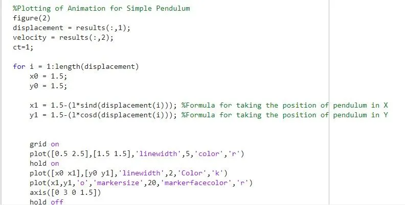
I didnt get a any error in the command window. But while I ran the program the motion of the simple pendulum is not that much as it will normally does. So I know that I did some mistake during programming. At that time I found out that, I provided sind() in the formula by providing radian in the input value. So I correct that command with normal sin() used for radian. After that the simulation looks perfect.

VIDEO LINK:

https://youtu.be/lbizlrOhIo0 , https://youtu.be/lbizlrOhIo0

RESULTS:
Thus we obtained the Velocity and Displacement curve as well as the animaition of the motion of a simple pendulum by solving the Second order ODE in matlab.