Week 4.1 - Genetic Algorithm

AIM:

To write a code to obtain the stalagmite function for the provided function and also to write a code of Genetic Algorithm to find out the global maxima for the particular stalagmite function.

OPTIMISATION:

Optimisation is a decision making process. It helps us to find a better results under set of prioritized constraints. The objective of the optimisation is to do multiple iterative process until the desired results will achieve. Optimisation techniques are categorised into four categories

1. Constrained Optimisation
2. Multimodal optimisation
3. Multi-objective optimisation
4. Combinatorial optimisation

The following procedure will processed to make the optimisation

Need for optimisation, Choose design variables, Formulate constraints, Formulate objective function, Set variable bounds, Chosse optimisation algorithm, obtain solution.

GENETIC ALGORITHM:

Genetic algorithm is one among the optimisation algorithm. It is the widely used optimisation algorithm as it is faster, and is used for multi-objective problems. The basic terminology of Genetic algorithm are as follows,

• Population - It is a subset of all the possible solution for the problem
• Chromosome - Chromosome is the one among the set of solution
• Gene - Gene is the one of the element of that solution
• Allele - Allele is the value of the particular element in that solution
• Genotype - Genotype is the computational space for solution. It is understandable and readable by the computer system
• Phenotype - Phenotype is the solution consists of Real world area. Where the solution is represented in Human readable format
• Encoding - It is the conversion of the solution from Phenotype to the Genotype
• Decoding - It is the conversion of the solution from genotype to the phenotype
• Fitness function - It is a function which will used to progress a input solution. It takes the input solution and provides the output. It verifies the fitness of the solution. Sometimes fitness function may also act as a objective function.
• Genetic Operators - It alters the offspring of the solution by using its operator named as cross over, mutation, selection.

SYNTAX FOR GA:

x = ga(fun,nvars,A,b,Aeq,beq,lb,ub,nonlcon,intcon,options)

This is the comman syntax for GA, whereas

The first element, func determines the function that we loaded for the GA. For eg: Stalagmite funciton

The second element, nvars, determines number of variables in the function.

The third and fourth element, A & b, indicates the value for the Inequality Linear functions

The fifth and sixth element, Aeq & beq, indicates the value for the equality linear functions

The seventh and eigth element, lb & ub, indicates the variable upper and lower bounds

The ninth element, nonlcon, indicates the value for the Inequality non linear functions

The tenth element, intcon, indicates the integer value involved in the function

The option element, has the various options that can be given to the GA like, tolerance, fitness limits, max generation, population size etc., Majorly used to terminate the conditions by provinding certain commands

TERMINATION CRITERIA FOR THE GA:

• Maxgeneration - algorithm stops when the number of generation reaches
• Maxtime - algorithm stops when the given time to evaluate the program
• Fitnesslimit - when it reaches the particular fitness limit mentioned
• Population size - When it reaches the pre determined population size

PROGRAM:

Program 1 - Stalagmite Function

function [f] = Stalagmite(input_vector)
x = input_vector(1);
y = input_vector(2);
Pi = 3.14;


f_a = (sin(5.1*Pi.*x+0.5)).^6;
f_b = (sin(5.1*Pi.*y+0.5)).^6;
A = -4*log(2);
B = ((x-0.0667).^2)/0.64;
C = ((y-0.0667).^2)/0.64;
f_c = exp(A*B);
f_d = exp(A*C);

f = - (f_a.*f_b.*f_c.*f_d) ;

end

Program 2 - Main Code

clear all
close all
clc

%Defining input variables
%Population Initializtaion

x = linspace(0,0.6,150);
y = linspace(0,0.6,150);

%Constraints for working space
Number_of_cases = 150;

%Conversion of 2D array

[xx,yy] = meshgrid(x,y);


%Function Definition
for i = 1:length(xx)
   for j = 1:length(yy)
        input_vector(1) = xx(i,j);
       input_vector(2) = yy(i,j);
    f(i,j) = Stalagmite(input_vector);
   end
end

%Study 1
%By providing the number of iteration does the GA run
%Random selection
tic  %to start the timer of the clock

for i=1:Number_of_cases
    [inputs,fopt(i)] = ga(@Stalagmite,2);
    xopt(i) = inputs(1);
    yopt(i) = inputs(2);
end
Studytime_1 = toc 


figure(1)
subplot(2,1,1) % command used to plot more than one plot in same figure
hold on
surfc(xx,yy,-f) %command which plots the surface in three dimension
shading interp
xlabel('X value')
ylabel('Y value')
zlabel('Function')
plot3(xopt,yopt,-fopt,'marker','o','markersize',5,'markerfacecolor','r') % command used to plot in three dimensional space
title('Unbounded Inputs')
subplot(2,1,2)
plot(-fopt)
xlabel('Iterations')
ylabel('Maximum Value')


%Study 2
%By providing the Upper bounds and Lower bounds


tic  %to start the timer of the clock

for i=1:Number_of_cases
    [inputs,fopt_2(i)] = ga(@Stalagmite,2,[],[],[],[],[0;0],[0.6;0.6]);
    xopt_2(i) = inputs(1);
    yopt_2(i) = inputs(2);
end
Studytime_2 = toc


figure(2)
subplot(2,1,1) 
hold on
surfc(xx,yy,-f) %command which plots the surface in three dimension
shading interp
xlabel('X value')
ylabel('Y value')
zlabel('Function')
plot3(xopt_2,yopt_2,-fopt_2,'marker','o','markersize',5,'markerfacecolor','r') % command used to plot in three dimensional space
title('Bounded Inputs')
subplot(2,1,2)
plot(-fopt_2)
xlabel('Iterations')
ylabel('Maximum Value')

disp('The value of X and Y to get the Maximum function')
X_Value = mean(xopt_2)
Y_Value = mean(yopt_2)
Function = mean(fopt_2)

%Study 3
%Increase the population size
tic  %to start the timer of the clock
options = optimoptions('ga')
options = optimoptions(options,'PopulationSize',500)
for i=1:Number_of_cases
    [inputs,fopt_3(i)] = ga(@Stalagmite,2,[],[],[],[],[0;0],[0.6;0.6],[],[],options);
    xopt_3(i) = inputs(1);
    yopt_3(i) = inputs(2);
end
Studytime_3 = toc

 
figure(3)
subplot(2,1,1)
hold on
surfc(xx,yy,-f) %command which plots the surface in three dimension
shading interp
xlabel('X value')
ylabel('Y value')
zlabel('Function')
plot3(xopt_3,yopt_3,-fopt_3,'marker','o','markersize',5,'markerfacecolor','r')% command used to plot in three dimensional space
title('Results after increasing population size')
subplot(2,1,2)
plot(-fopt_3)
xlabel('Iterations')
ylabel('Maximum Value')

disp('The value of X and Y to get the Maximum function')
X_Value1 = mean(xopt_3)
Y_Value2 = mean(yopt_3)
Function1 = mean(fopt_3)

CODE EXPLANATION:

• Initially I define the variables using linspace() command for x and y. Then i convert the one dimensional array in to two dimensional array using meshgrid() command. Then I provide the number of cases value for providing the iteration time that the GA should run for the function.
• Then I define the stalagmite function that I already coded seperately for the value of x and y in the for loop, that will look upon every element in xx and yy. And the output results is stored in the f.
• Then the Study 1 is started. In this study, we allowed the random selection of the search base. Then we use the pre-defined function ga() and inside that we use our stalagmite funciton. And the outcome is stored as fopt,xopt and yopt.
• After that, we use the subplot() command to show the various plots inside the single figure. Then we use the surfc() to show case the surface of the stalagmite function. Then we use the plot3() command,to mark the plot in three dimensional space. And Seperately we plot the fopt in seperate plot and merged in the same figure using subplot() command.
• In this we are using the tic and toc command to measure the time taken for the study 1.
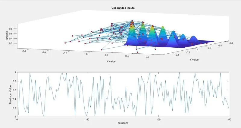
• And in the end we observed that we are getting lot number of maximum position due to the random selection of the variables alloted to the x and y.
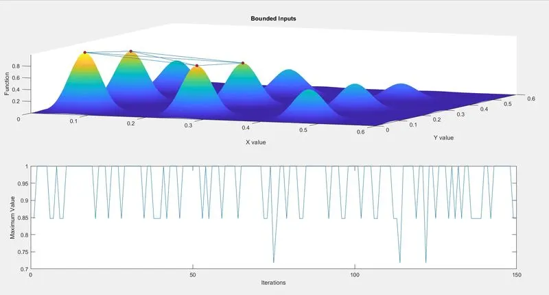
• Then in the study 2 , inside the ga() function we fixed the inbounds and outbounds to the search base. So that random selection of the function is avoided. And we instruct the algorithm to follow the search base of what we provided it to.
• Then similarly plotting is done. After providing the variable bounds , it is clearly seen that within the bounds the ga calculate the global maximum . But it shows four maximum. So out of those it is tedious to find out the maximum position.
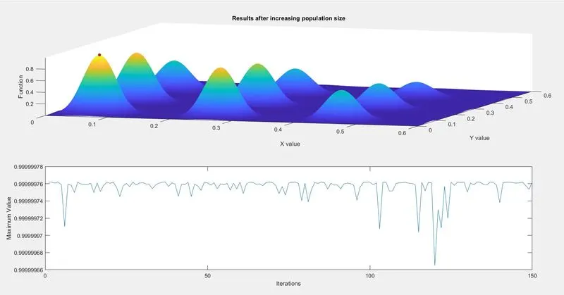
• So for that case study 3 is initiated, in this we are providing the population size. This will enhance the ga algorithm to provide the fittest member. But it will take a lot of time to complete it as many iterations have to take place.
• But we can get a accurate results out of it.

PLOT:

Plot 1 - Random selection of input variables

Plot 2 - Bounded Variables given

Plot 3 - Population size is given

RESULTS:

Thus by using the Genetic Algorithm (optimisation tool), We optimise the stalagmite function.

The value of X and Y to get the Maximum function

X_Value1 =

0.0669

Y_Value2 =

0.0669

The Function results is 0.999999665

REFERENCES:

• Wikipedia
• Youtube surfing
• Genetic Algorithms Tutorial (tutorialspoint.com)
• Mathworks