Project 2 - Rankine cycle Simulator

AIM:

To create a Rankine Simulator using the Matlab. To write a code to calculate the state points in each of the processes based upon the user input. With respect to that, to find out the state variables between those state points with the help of thermodynamic relation. And to plot the T-S and H-S plots with the user defined inputs.

WORKING PRINCIPLE:

In general, the Rankine cycle is an idealized thermodynamic cycle of a constant pressure heat engine that converts part of heat into mechanical work. In this cycle the heat is supplied externally to a closed loop, which usually uses water (in a liquid and vapour phase) as the working fluid. The working fluid in the Rankine cycle undergo the phase change from a liquid to vapour phase and vice versa.

One of the major advantages of the Rankine cycle is that the compression process in the pump takes place on a liquid. By condensing the working steam to a liquid (inside a condenser) the pressure at the turbine outlet is lowered and the energy required by the feed pump consumes very much lesser than of the turbine output power and these factors contribute to a higher efficiency for the cycle.

The processes that the rankine cycle covers is of Isentropic compression, Isobaric heat addition, Isentropic expansion and Isobaric heat rejection process. Lets discuss with these process in brief

Isentropic Expansion:(1-2)

• Enthalpy decreases as the work done by the turbine.
• Temperature and pressure also decreases due to the expansion of saturated steam .
• Entropy of the process remain constant as the isentropic process happens.

Isobaric heat rejection:(2-3)

• Heat rejection happens due to the heat transfer to the outer system using condenser to the minimal. Phase change also happens by this time as the conderser condensate the vapour into liquid.
• Pressure remains constant through out this process.

Isentropic Compresssion:(3-4)

• Here the water is compresser isentropically using the water pump. Hence the entropy remains constant.
• Pressure and enthalpy of the system increases as the work done by the pump to the working fluid.

Isobaric heat addition:(4-1)

• Heat addition happens by the heat transfer using the heat exchanger. Temperature of the working fluid increases with the slight increase of enthalpy.
• Pressure is assumed to be constant throughout this process as it states isobaric.

Net work done by the system:

During a Rankine cycle, work is done on the fluid by the pumps between states 3 and 4 (isentropic compression). Work is done by the fluid in the turbine between stages 1 and 2 (isentropic expansion). The difference between the work done by the fluid and the work done on the fluid is the net work produced by the cycle .

Efficiency:

In general the Thermal efficiency of rankine cycle is defined as the ratio of the work it does , to the heat input at the high temperature.

PROGRAM:

clear
close all
clc

% to display the header
disp('                Rankine Cycle Stimulator                ')


% to display the process  flow
disp('Process 1 - 2 - Isentropic expansion process happens in the turbine') 
disp('Process 2 - 3 - Isobaric heat rejection process takes place in the condenser')
disp('Process 3 - 4 - Isentropic compression process happens in the pump')
disp('Process 4 - 1 - Isobaric Heat addition process takes place in the Heat Exchanger')

%Collection of inputs from the user
T1 = input('The Turbine inlet temperature, T1(in C) = ');
P1 = input('The Turbine inlet pressure, P1 (in bar)= ');
P2 = input('The Turbine outlet pressure, P2 (in bar) = ');

%Calculation of  state point 1

H1 = XSteam('h_pT',P1,T1);
S1 = XSteam('s_pT',P1,T1);
Hl1 = XSteam('hL_p',P1);
Hg1 = XSteam('hV_p',P1);
Sl1 = XSteam('sL_p',P1);
Sg1 = XSteam('sV_p',P1);
T_sat1 = XSteam('Tsat_p',P1);

%Calculation of state point 2

S2=S1;
Sl2 = XSteam('sL_p',P2);
Sg2 = XSteam('sV_p',P2); 
Hl2 = XSteam('hL_p',P2);
Hg2 = XSteam('hV_p',P2);
X = (S2-Sl2)/(Sg2-Sl2);
H2 = ((Hg2-Hl2)*X) + Hl2; % X = (H2-Hl2)/(Hg2-Hl2)
T2 = XSteam('T_ps',P2,S2);
T_sat2 = XSteam('Tsat_p',P2);  

%Calculation of state point 3

P3 = P2;
S3 = XSteam('sL_p',P3);
H3 = Hl2;
T3 = XSteam('T_ps',P3,S3);

%Calculation of state point 4

S4 = S3;
P4 = P1;
T4 = XSteam('T_ps',P4,S4);
H4 = XSteam('h_ps',P4,S4);

%Calculation of other parameters

W_Turb = H1 - H2; %Work done by the turbine

W_Pump = H4 - H3; %Work done by the pump

Q_Htexch = H1 - H4; %Heat given to the system

W_Output = W_Turb - W_Pump; %Total Work output of the system

Efficiency = (W_Output / Q_Htexch) * 100 ; %Efficiency of the cycle

Back_Ratio = W_Pump/W_Turb;

SSC = 3600 / W_Turb;

% Displaying Results in the Command Window

% To display State point 1 results
disp('             RESULTS             ')
disp('State point 1')

fprintf('\nTemperature at 1 is  : %.2f degree celcius \n',T1);
fprintf('Pressure at 1 is : %.2f bar \n',P1);
fprintf('Enthalpy at 1 is : %.2f kJ/Kg\n',H1);
fprintf('Entropy at 1 is : %.2f kJ/KgK\n\n',S1);

%To display state point 2 results
disp('State point 2')

fprintf('\nTemperature at 2 is  : %.2f degree celcius \n',T2);
fprintf('Pressure at 2 is : %.2f bar \n',P2);
fprintf('Enthalpy at 2 is : %.2f kJ/Kg\n',H2);
fprintf('Entropy at 2 is : %.2f kJ/KgK\n\n',S2);

%To display state point 3 results
disp('State point 3')

fprintf('\nTemperature at 3 is  : %.2f degree celcius \n',T3);
fprintf('Pressure at 3 is : %.2f bar \n',P3);
fprintf('Enthalpy at 3 is : %.2f kJ/Kg\n',H3);
fprintf('Entropy at 3 is : %.2f kJ/KgK\n\n',S3);

%To display state point 2 results
disp('State point 4')

fprintf('\nTemperature at 4 is  : %.2f degree celcius \n',T4);
fprintf('Pressure at 4 is : %.2f bar \n',P4);
fprintf('Enthalpy at 4 is : %.2f kJ/Kg \n',H4);
fprintf('Entropy at 4 is : %.2f kJ/KgK \n\n',S4);

fprintf('Turbine work output is : %.2f kJ/kg\n',W_Turb); % To display Turbine work output
fprintf('Pump Work output is : %.2f kJ/kg \n',W_Pump); % To display pump work output
fprintf('Net Work output is : %.2f kJ/kg \n',W_Output); % To display Net work output
fprintf('Efficiency of cycle is : %.2f\n',Efficiency); % To display efficiency of cycle
fprintf('Specific Steam Consumption is : %.2f kg/kWh \n',SSC); % To display specific steam consumption
fprintf('Back Work Ratio is : %.4f \n',Back_Ratio); % To display the  back work ratio

%Plotting of TS diagram 
%Plotting of TS curve

T = linspace(0,393.94,500);
figure(1)
hold on
grid on
for i = 1:length(T)
    plot(XSteam('sL_T',T(i)),T(i),'g.')
     plot(XSteam('sV_T',T(i)),T(i),'g.')
end

plot([S1 S2],[T1 T2],'linewidth',3,'color','k')
text(S1,T1+50,'1','FontSize',10)
if X>1
T3 = T_sat2;
plot([S2 S_g2 S3 S4],[T2 T_sat2 T3 T4],'linewidth',3,'color','b')
T2 = T_sat2;
text(S2+1,T2,'2','FontSize',10)
text(S3,T3+30,'3','FontSize',10)
else
plot([S2 S3 S4],[T2 T3 T4],'linewidth',3,'color','b')
text(S2+1,T2,'2','FontSize',10)
text(S3,T3+30,'3','FontSize',10)
end

n = linspace(T1,T2,500);
for i = 1:length(n)
plot(XSteam('s_pT',P1,n(i)),n(i),'.','linewidth',3,'color','r')
end

plot([Sl1 Sg1],[T_sat1 T_sat1],'linewidth',3,'color','k')
text(Sl1,T_sat1+30,'4','FontSize',10)
xlabel('Entropy(kJ/kg-K)')
ylabel('Temperature(K)')
axis([0 10 0 500])
title('T-S Plot')

%Plotting of HS Diagram
%Plotting of HS  Curve
figure(2) 
hold on
grid on
for i = 1:length(T)
 plot(XSteam('sL_T',T(i)),XSteam('hL_T',T(i)),'b.')
 plot(XSteam('sV_T',T(i)),XSteam('hV_T',T(i)),'b.')
end
plot([S1 S2 S3 S4 S1],[H1 H2 H3 H4 H1],'linewidth',3,'color','k')
text(S1+0.5,H1,'1','FontSize',10)
text(S2+0.5,H2,'2','FontSize',10)
text(S3+0.5,H3,'3','FontSize',10)
text(S4,H4+150,'4','FontSize',10)
xlabel('Entropy(kJ/kg-K)')
ylabel('Enthalpy(kJ/kg)')
title('H-S PLOT')

CODE EXPLANATION:

• To predefined the structure of the rankine cycle and its processes to the user, I use display() command to display the process informations from 1-4.
• Then to collect the user input into the program for further calculation I use fprintf() command to collect the data of Temperature and Pressure at state point 1 and Pressuure at the state point 2. Using these inputs the program is written to collect the required datas.
• The important data necessary for the calculation is taken from XSteam library basically a steam table, where we can collect the data for the state points.
• Then using the XSteam table, I collect all the data necessary for the calculations include all the state points values.
• After that using the thermodynamic relation, I find out the efficiency and the state variables for the Rankine cycle.
• Then I did the plotting with the help of the state points collected using Xsteam library.
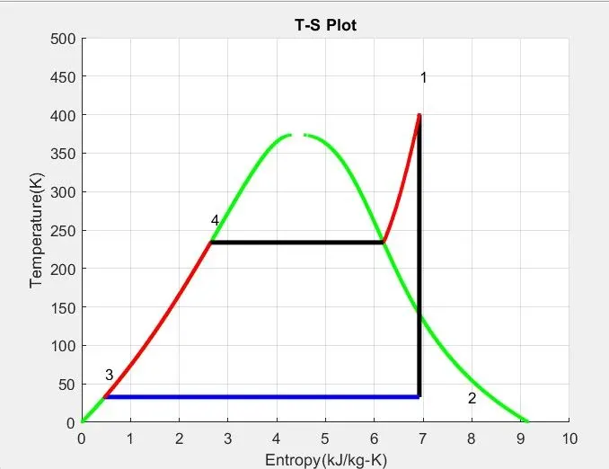
• Here TS curve is drawn before proceeding to plot the state points. The TS curve is drawn to the entropy for the critical temperature for the water with respect to its temperature.
• By considering the dryness fraction of the steam, we plot the TS value in the plot.
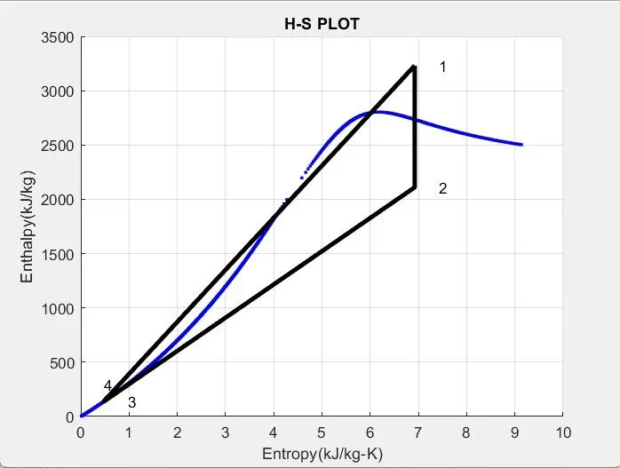
• Then for the HS curve, I considered the value of enthalpy and entropy for the temperature that is range maximum to the critcal temperature of the water.
• Then I plot the values of the H and S state points in the plot to obtain the relation.

PLOT:

Plot 1 - TS plot:

Plot 2 - HS plot:

RESULTS:

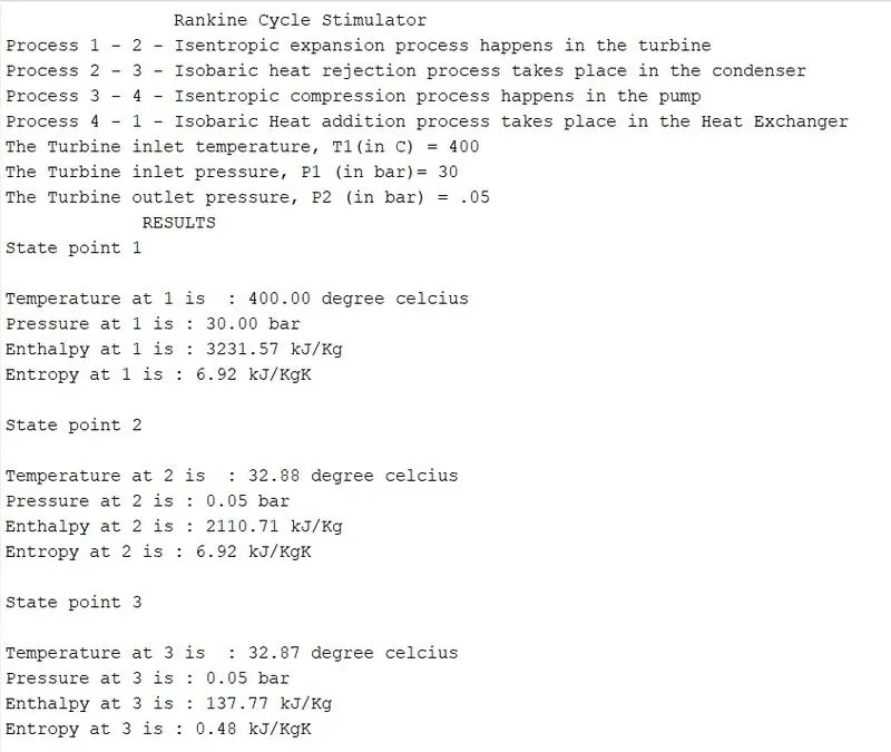
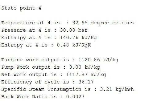
Thus the program is created and executed using the user defined data to calculate the state points and also the state variables of the Rankine cycle. And also the plots for the relevant user input data has plotted using the matlab program code.