Auto ignition using Cantera

Can we burn something without fire?

Yes. The essential components required for burning something are Fuel, an oxidizer, and a Heat source. Fire is one of a kind of heat source, but not the only one. Thus, we can burn stuff without fire.

In fact, one of the most common auto-mobile engines called the Diesel Engine does not have a spark plug. Instead, the Fuel is Auto-ignited because of the high temperature. The minimum temperature required for the Auto-ignition of fuel is called the Auto-Ignition temperature.

Once the Auto-ignition temperature is attained, after a very short time, the fuel auto-ignites. The short time required for the ignition of the fuel is called the Ignition Delay.

Aim

This project aims to find the dependence of the Ignition Delay of Methane on the Initial temperature and Pressure of the Mixture using Python and Cantera.

Code and its explanation:

Libraries required :

Finding Ignition Delay involves solving fundamental governing equations related to fluids and to increase the complexity, we also have to solve the species equation. Writing a program to do this is a very time-consuming job.

Luckily, there is a Library that can help us find the ignition delay easily. Apart from ignition delay, this library can do a lot of other crazy stuff. The library is called Cantera. To read more about Cantera - click here Cantera .

The other libraries required for this project are Matplotlib for plotting and Numpy (Added incase any array-related operations are to be performed).

import cantera as ct
import numpy as np
import matplotlib.pyplot as plt

Function:

• This function takes the initial temperature, pressure, and species concentration as inputs and provides temperature, species concentration at each timestep and the ignition delay as the output
• We first call the Class Solution as gas and import the solution mechanism file gri30.yaml
• Provide initial temperature, pressure, and species concentration to gas using gas.TPX
• The idealgasreactor class has all the governing equations required to obtain different states, properties, and other variables in the reaction.
• The ReactorNet is used to couple all the reactors for simultaneous reactions. In this case, we have only one reactor. But it is mandatory to use the ReactorNet class.
• The SolutionArray class stores the solution at each instant in time.
• Define time - It is ideal to use total time in such a way that the relative difference between the ignition delay and the total time must not be huge. This is done to keep plots easily readable and also save computational time.
• The advanced class is used to advance the timesteps. It is placed in a while loop, to keep advancing timesteps until the end time is reached.
• The ignition temperature for this problem is defined as the Initial temperature+400. A for-if loop is included to find the timestep at which the ignition temperature is attained.
• The function returns the output values defined in point one.

def ignitionDelay(T,P,species):
    gas=ct.Solution('gri30.yaml')
    gas.TPX=T,P,species
    
    r=ct.IdealGasReactor(gas)    
    sim=ct.ReactorNet([r])

    states=ct.SolutionArray(gas,extra= 't') 

    totalTime = 10

    while sim.timeT+400:
            
            tdindex.append(i)
            
    delaytimestep=tdindex[0]
    delay=states.t[delaytimestep]

    return states.t, states.T, states.X, delay

Species

species={'CH4':0.095,'O2':0.19011,'N2':0.71482}

PART 1

Plot the variation of the Auto Ignition time of Methane with a constant temperature of 1250K and pressure varying from 1 to 5 atm.

A Total time of 0.1 sec is sufficient in this case to capture the ignition process.

Code

The code uses straightforward commands and is self-explanatory.

plt.title("Initial Temperature = 1250k")

plt.plot(ignitionDelay(1250,101325,species)[0],ignitionDelay(1250,101325,species)[1])

plt.plot(ignitionDelay(1250,2*101325,species)[0],ignitionDelay(1250,2*101325,species)[1])

plt.plot(ignitionDelay(1250,3*101325,species)[0],ignitionDelay(1250,3*101325,species)[1])

plt.plot(ignitionDelay(1250,4*101325,species)[0],ignitionDelay(1250,4*101325,species)[1])

plt.plot(ignitionDelay(1250,5*101325,species)[0],ignitionDelay(1250,5*101325,species)[1])

plt.legend(["P=1 atm, Ignition Delay = " + str(round(ignitionDelay(1250,101325,species)[2],4)) + " sec",
            "P=2 atm, Ignition Delay = " + str(round(ignitionDelay(1250,2*101325,species)[2],4)) + " sec",
            "P=3 atm, Ignition Delay = " + str(round(ignitionDelay(1250,3*101325,species)[2],4)) + " sec",
            "P=4 atm, Ignition Delay = " + str(round(ignitionDelay(1250,4*101325,species)[2],4)) + " sec",
            "P=5 atm, Ignition Delay = " + str(round(ignitionDelay(1250,5*101325,species)[2],4)) + " sec"],loc ="lower right")

plt.xlabel("Time (sec)")
plt.ylabel("Temeprature (k)")
plt.grid()
plt.show()

Output:

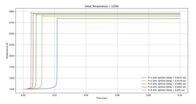
Inference

• As the pressure increases, the ignition delay time decreases. The possible reason for this can be the intermolecular distances. At higher pressure, the intermolecular distance is less, i.e. the density of the gas is high. This leads to faster heat transfer and thus lower ignition delay time.

Plot the variation of the Auto Ignition time of Methane with a constant pressure of 5 atm and temperature varying from 950K to 1450K.

Note: Since the initial temperature is low in one of the cases of this part. We have to increase the total time to capture the ignition for those cases. A sufficient total time would be 0.5 sec.

Code

plt.title("Initial Pressure = 5 atm")

plt.plot(ignitionDelay(950,5*101325,species)[0],ignitionDelay(950,5*101325,species)[1])

plt.plot(ignitionDelay(1050,5*101325,species)[0],ignitionDelay(1050,5*101325,species)[1])

plt.plot(ignitionDelay(1150,5*101325,species)[0],ignitionDelay(1150,5*101325,species)[1])

plt.plot(ignitionDelay(1250,5*101325,species)[0],ignitionDelay(1250,5*101325,species)[1])

plt.plot(ignitionDelay(1350,5*101325,species)[0],ignitionDelay(1350,5*101325,species)[1])

plt.plot(ignitionDelay(1450,5*101325,species)[0],ignitionDelay(1450,5*101325,species)[1])

plt.legend(["T=950 K, Ignition Delay = " + str(round(ignitionDelay(950,5*101325,species)[2],4)) + " sec",
            "T=1050 K, Ignition Delay = " + str(round(ignitionDelay(1050,5*101325,species)[2],4)) + " sec",
            "T=1150 K, Ignition Delay = " + str(round(ignitionDelay(1150,5*101325,species)[2],4)) + " sec",
            "T=1250 K, Ignition Delay = " + str(round(ignitionDelay(1250,5*101325,species)[2],4)) + " sec",
            "T=1350 K, Ignition Delay = " + str(round(ignitionDelay(1350,5*101325,species)[2],4)) + " sec",
            "T=1450 K, Ignition Delay = " + str(round(ignitionDelay(1450,5*101325,species)[2],4)) + " sec",],loc ="lower right")

plt.xlabel("Time (sec)")
plt.ylabel("Temeprature (k)")
plt.grid()
plt.show()

Output:

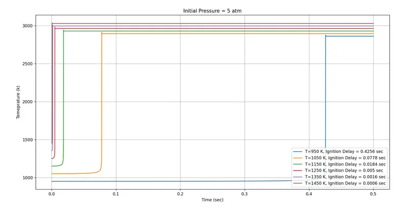
• As Temperature increases, the ignition delay time decreases. This is intuitive as higher the temperature faster is the ignition.

PART II :

Further, observe and print the rate of change of molar concentrations of the given elements "H2O, O2, OH" with respect to the time, (simulation time = 10 secs)

Explain the behavior of the graph for 2 cases,

• When the Temperature is 1000K and the pressure 5 bar
• When the Temperature is 500K and the pressure 5 bar

Combustion of Methane is not a single reaction, it involves a lot of intermediaries reactions and thus involves lot of species. state.X would give us mole fractions of all the species available at the specific time step.

We use the species_names command inbuild in the Cantera library to find the index number at which the species we desire to study are present. For example, O2 is at an index number of 3.

Code:

ig=ignitionDelay(1000,5*101325,species)

plt.title("Initial Pressure = 5 atm, Temperature = 1000 K")

plt.plot(ignitionDelay(1000,5*101325,species)[0],ignitionDelay(1000,5*101325,species)[2][:,13])
plt.plot(ignitionDelay(1000,5*101325,species)[0],ignitionDelay(1000,5*101325,species)[2][:,5])
plt.plot(ignitionDelay(1000,5*101325,species)[0],ignitionDelay(1000,5*101325,species)[2][:,3])
plt.plot(ignitionDelay(1000,5*101325,species)[0],ignitionDelay(1000,5*101325,species)[2][:,4])

plt.legend(["CH4","H2O","O2","OH"],loc ="lower right")

plt.xlabel("Time (sec)")
plt.ylabel("Concentration")
plt.grid()
plt.show()

Output for T = 1000k and 5 bar.

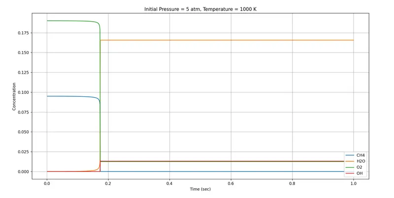
Inference:

• The species present on the reactant side of the stoichiometric reaction are consumed once the mixture is ignited and thus they have lower concentrations after ignition.
• The species which are formed or are products are increased after the ignition process is started.

output at T=500 K and P=5 bar.