Week 7 - Auto ignition using Cantera

Auto-ignition time delay with varying temperature and pressure:

The auto-ignition time delay is the time taken for the mixture to reach a tempeture of 400 [K] greater then the initial temperature. This parameter is very important fuel property since it determines the ability to start the combusiton of a fuel rapidly. Such as in diesel engines, diesel is expected to auto ignite within a very short time-period after injection into the hot compressed air. If the auto-ignition delay increases due to impurities, it could cause misfirings and serious damage. In the current case, stoichiometric amount of air and methane are let to auto-ignite at various initial pressure and temperature conditions. The effect of pressure changes at constant temperature and the effects of temperature at constant pressure on auto-ignition time delay are analysed. A python program using cantera is used to determine the auto-ignition time delay. A function is written to take in the initial temperature, pressure, species mole fraction and time array with the time values to be solved for. The function creates a solution object based on gri30.xml, initial conditions for the solution object are set, a new reactor of ideal gas type is added with the solution object and reactor network is also added for this reactor. The method advance() in reactor network is used to integrate the reactor to the time-limit specified. The time integration is continued until auto-ignition temperature is reached and the time-taken is returned by the function. The program solves this problem in 2 steps. In first step, temperature is fixed to 1250 [k] and pressure is varied from 1 [atm] to 5 [atm]. For each value of pressure, the ignition time delay is calculated using the function. Similarly, in second step, pressure is kept constant at 5 [atm] and temperature is varied from 950 [K] to 1450 [K] and auto-ignition time-delay is computed. Results are plotted using matplotlib.

'''
Simulation of autoIgnition time delay for methane  
plot the effect of pressure and temperature
'''

import numpy as np
import matplotlib.pyplot as plt
import cantera as ct

t0 = 0.0 									# initial time
tmax = 10									# final time
dt = 1e-3									# time-step size
time_arr = np.arange(t0,tmax+dt,dt)			# time array


def autoIgnition_delay(T, P, species_dict, time_arr):
	# function to calculate autoIgnition time delay
	gas = ct.Solution("gri30.xml")
	gas.TPX = T, P, species_dict
	r = ct.IdealGasReactor(gas)
	sim = ct.ReactorNet([r])
	states = ct.SolutionArray(gas,extra=["time_in_ms","t"])

	for time in time_arr:
		# loop over time values
		sim.advance(time)
		states.append(r.thermo.state, time_in_ms = time * 1e3, t = time)
		if r.T >= T + 400:
			# step when auto-ignition temperature is reached - note the time delay
			delay = time * 1e3
			break
	return delay


## constant temperature and variable pressure
T = 1250 															# temperature
P_arr = np.linspace(1,5,20)											# pressure array
species_dict = {"CH4":1,"O2":2,"N2":7.52}							# species mole fraction
delay_arr = np.zeros(len(P_arr))									# result array for auto-ignition time delay

for i in range(len(P_arr)):
	# calculate auto-ignition time delay for different pressures
	P = P_arr[i] * 101325
	delay_arr[i] = autoIgnition_delay(T,P,species_dict,time_arr)

# plot result
plt.figure(1)
plt.plot(P_arr,delay_arr)
plt.title("Pressure vs Auto-Ignition-delay")
plt.xlabel("Pressure [atm]")
plt.ylabel("Auto Ignition delay [ms]")

## constant pressure and variable temperature
P = 5 * 101325 													# pressure
T_arr = np.linspace(950,1450,20)								# temperature array
species_dict = {"CH4":1,"O2":2,"N2":7.52}						# species mole fraction
delay_arr = np.zeros(len(T_arr))								# result array for auto-ignition time delay

for i in range(len(T_arr)):
	# calculate auto-ignition time delay for different temperatures
	T = T_arr[i] 
	delay_arr[i] = autoIgnition_delay(T,P,species_dict,time_arr)

# plot result
plt.figure(2)
plt.plot(T_arr,delay_arr)
plt.title("Temperature vs Auto-Ignition-delay")
plt.xlabel("Temperature [K]")
plt.ylabel("Auto Ignition delay [ms]")
plt.show()

Results:

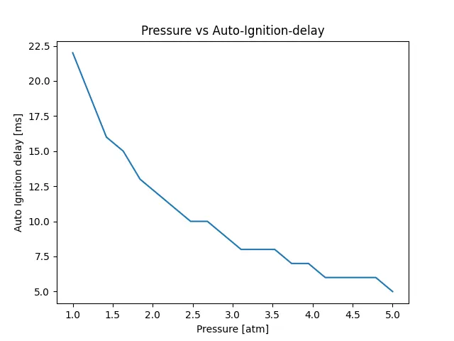
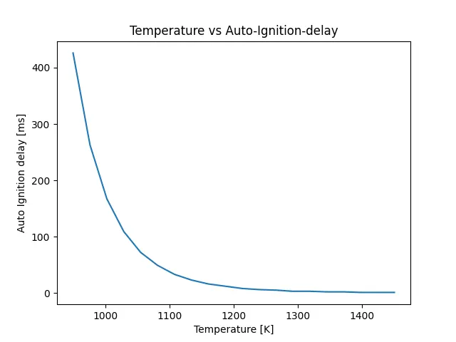
From the plots, it can be clearly seen that the auto-ignition time delay is a function of system pressure and temperature. The effect of temperature is much more than pressure. With increased pressure, the particles are packed more closer to each other enabling better chance of reaction. With increased temperature, the mean particle velocity is increased and hence the chances of particles colliding with each other to make the reaction happen are higher. With temperature rise from 950 [K] to around 1100 [K], the gradient of ignition time delay is very strong and slowly this rate reduces with increase in temperature. Increase in pressure also facilitates reduction in ignition time delay, however the scale of this change is much smaller compared to temperature variation.

Variation of species mole fraction with temperature:

When the solution advances through time, the species mole fraction in the reactor varies as per the reactions and their reaction rates. Monitoring the rate of change of some species gives an idea about the combustion progress and process. Here the evolution of mole fraction of species, `H_2O, O_2 and OH` are monitored. `H_2O` being on the product side of combustion process indicates product production rate. `O_2` being on the reactants side of combustion specifies the rate of usage of oxygen and the remaining oxygen for combustion in the reactor. `OH` being the intermediatory species, show if the combustion is in progress and complete combustion is achieved. Here, these species mole fractions are monitored for a couple of cases with a pressure of 5 [atm] and temperatures of 500 [K] and 1000 [K]. A python program similar to previous one is written for this simulation. A SolutionArray object is created to store the reactor thermal properties at every time step that we specify. Then the evolution of particular species mole fractions over time are obtained from the SolutionArray and plotted against time for the 2 temperature options specified.

'''
Simulation of autoIgnition of methane 
plot the gradients of species
'''

import numpy as np
import matplotlib.pyplot as plt
import cantera as ct

t0 = 0.0												# initial time
tmax = 10												# final time
dt = 1e-3												# time-step size
time_arr = np.arange(t0,tmax+dt,dt)						# time array

def autoIgnition_delay(T, P, species_dict, time_arr):
	# function to simulate autoIgnition
	gas = ct.Solution("gri30.xml")
	gas.TPX = T, P, species_dict
	r = ct.IdealGasReactor(gas)
	sim = ct.ReactorNet([r])
	states = ct.SolutionArray(gas,extra=["time_in_ms","t"])

	for time in time_arr:
		# loop over time values
		sim.advance(time)
		states.append(r.thermo.state, time_in_ms = time * 1e-3, t = time)
	
	# save and return evolution of species mole fraction
	H2O_X = states.X[:,gas.species_index('H2O')]
	O2_X = states.X[:,gas.species_index('O2')]
	OH_X = states.X[:,gas.species_index('OH')]
	return [H2O_X, O2_X, OH_X]


P = 5 * 101325 										# pressure
T_arr = [500, 1000]									# temperature array
species_dict = {"CH4":1,"O2":2,"N2":7.52}			# species mole fraction

j = 1												# plot counter
for i in range(len(T_arr)):
	# Loop over the temperature inputs 
	T = T_arr[i] 

	# calculate evolution of species fraction for T
	[H2O_X, O2_X, OH_X] = autoIgnition_delay(T,P,species_dict,time_arr)

	# plot results
	plt.figure(i+j)
	plt.plot(time_arr,H2O_X)
	plt.title("Time vs H2O-mole-fraction, T=%i" %T)
	plt.xlabel("Time [s]")
	plt.ylabel("H2O-mole-fraction")
	j+=1

	plt.figure(i+j)
	plt.plot(time_arr,O2_X)
	plt.title("Time vs O2-mole-fraction, T=%i" %T)
	plt.xlabel("Time [s]")
	plt.ylabel("O2-mole-fraction")
	j+=1

	plt.figure(i+j)
	plt.plot(time_arr,OH_X)
	plt.title("Time vs OH-mole-fraction, T=%i" %T)
	plt.xlabel("Time [s]")
	plt.ylabel("OH-mole-fraction")

plt.show()

Results:

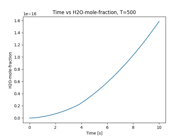
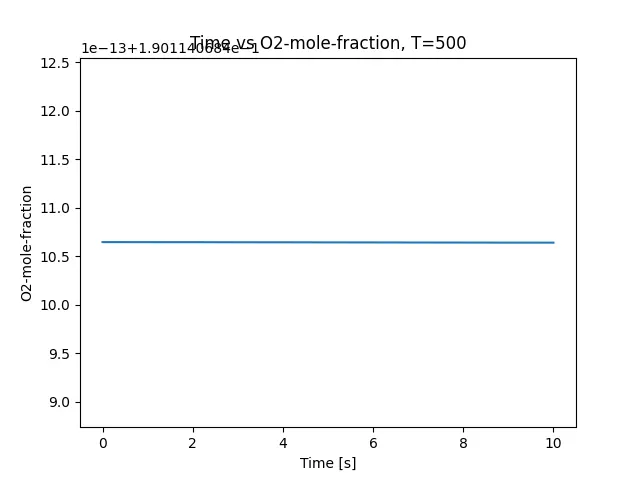
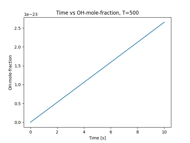
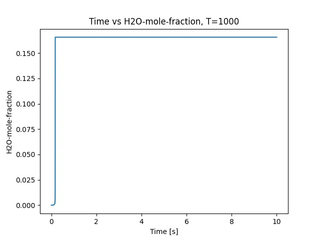
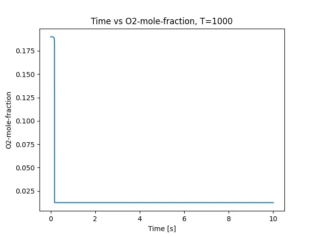
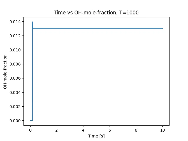
For the case with 500 [K], `H_2O` mole fraction seems to increase, but in negligible amount. `O_2` mole fraction seems to almost constant. `OH` mole fraction is increasing which means the intermediatory reactions are in progress, but the production rates of `OH` is in negligible amount. So, considering the changes in `H_2O` and `OH`, which are in the order of 1e-16 and 1e-23, negligible, the mixture can be assumed to be in equilibrium and auto-ignition will not happen. For the second mixture at 1000 [K], it can be seen that the `H_2O` mole fraction rises rapidly at a few milliseconds and reaches a constant level when the mixture attains equilibrium. Similarly, `O_2` mole fraction suddenly drops at few milliseconds where auto-ignition starts and reaches a constant value where the mixture reaches equilibrium. The evolution of `OH` shows the rate of intermediatory reactions during combustion. It rises rapidly after auto-ignition, reaches a maximum and then drops to equilibrium conditions.