Week 7 - Auto ignition using Cantera

AIM: To simulate auto-ignition time and molar concentration of the elements for methane using the reactor network code.

OBJECTIVE:

• To plot the variation of Auto Ignition time of Methane with a constant temperature of 1250K and pressure varying from 1 to 5 atm.
• To plot the variation of Auto Ignition time of Methane with a constant pressure of 5 atm and temperature varying from 950K to 1450K.

• To observe and print the rate of change of molar concentrations of the given elements "H2O, O2, OH" with respect to the time, (simulation time = 10 secs)

Explain the behavior of the graph for 2 cases,

• When Temperature is 1000K and pressure 5 bar
• When Temperature is 500K and pressure 5 bar

Auto-ignition:The spontaneous ignition of fuel and oxidizer mixture in the absence of any external ignition source.

• The increasing radical concentration leads to increase in reaction rate build on themselves,and results in an ignition through a rapid explosive rise in radical concentration,oxidation rate and temperature.

An auto-ignition delay time of fuels is defined as the time interval required for fuel -air mixture to spontaneously ignite at some conditions.

• RCM(Rapid compression machine) and shock tubes are used to study ignition delay time.
• Shock tube is applied to study ignition delay time at higher temperature and pressure.
• RCM measures the ignition delay time by simulating the process of adiabatic compression and ignition.

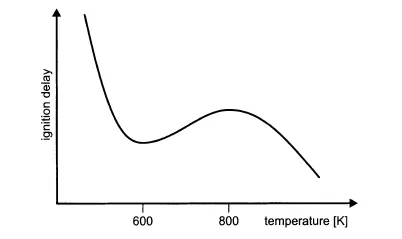
Fig. Negative temperature coefficient for hydrocarbon ignition

• The above graph shows the negative temperature region i.e, in temperature range of 600k to 800 k, where the ignition delay increases as the temperature increases.
• In all other temperature region,the trend of ignition delay decreases as the temperature increases.
• For modelling of low temperature combustion models,it is very challenging to model as the low temperature region is very narrow(400-700) where the ignition delay time is minimum.
• Some precautions taken for LTC models, as the emissions tends to increases in these regime.

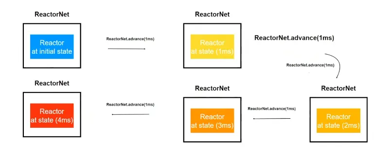
Fig. Schematic view of instance of reactor state.

• In this case,a gas object is created from solution class,so that the input conditions are temp,pressure and molar concentration.
• A reactor object is choosen as it represents a chemically reacting system in which all state variables are uniformly distributed.
• Then we have defined ideal gas reactor model as it takes the temperature as state variable instead of internal energy.
• ReactorNet.advance is used as a command for moving the time step forward from 1ms to 5ms (say).

case1: Auto ignition time with constant temperature and pressure varying from 1 to 5 atm.

import sys
import numpy as np
import cantera as ct
import matplotlib.pyplot as plt
gas=ct.Solution('gri30.xml')
Press=[]
ignition_time=[]
T1=1250
for P1 in range(1,6,2):
	P=P1*101325
	print(P)
	gas.TPX=T1,P,{'CH4':1,'O2':2,'N2':7.52}
	r=ct.IdealGasReactor(gas)
	sim=ct.ReactorNet([r])
	time=0.0
	states=ct.SolutionArray(gas,extra=['t'])
	for i in range(10000):
		time=time+1e-3
		sim.advance(time)
		states.append(r.thermo.state,t=time)
		if (states.T[i]<=(T1+400)):
			t_1=(states.t[i])
			pressure=(states.P[i])
			
	ignition_time.append(t_1)
	Press.append(pressure)


	plt.figure(1)
	plt.plot(states.t,states.P,label='initial pressure=%s'%P1)
	plt.title("Pressure vs time")
	plt.xlabel('time(sec)')
	plt.legend()
	plt.ylabel('pressure(Pa)')

#ignition_time.append(t_1)
#Temp.append(temp)

	
plt.figure(2)
plt.plot(Press,ignition_time,'*',color='blue')
plt.plot(Press,ignition_time)
plt.title('ignition delay vs pressure')
plt.xlabel('pressure(pa)')
plt.ylabel('ignition_delay_time')
plt.show()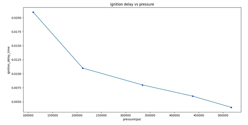

Fig.1 Ignition_delay_time vs pressure

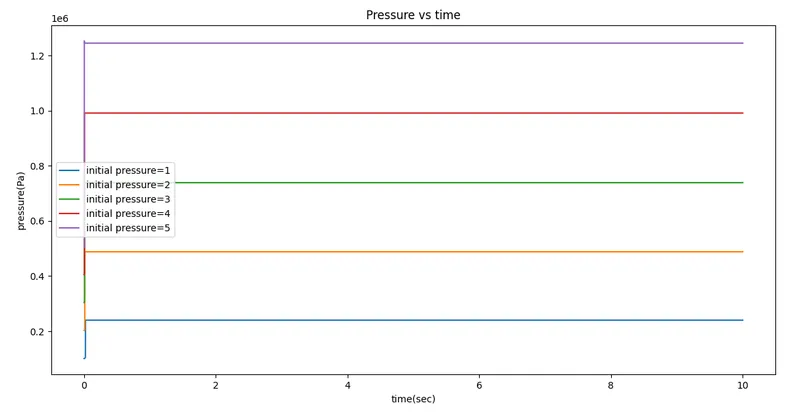
Fig.2 Pressure vs time

case2: Auto ignition time with constant pressure and temperature varying from 950k to 1450k.

import sys
import numpy as np
import cantera as ct
import matplotlib.pyplot as plt
gas=ct.Solution('gri30.xml')
Temp=[]
ignition_time=[]

for T1 in range(950,1550,100):
	P=5*101325
	print(T1)
	gas.TPX=T1,P,{'CH4':1,'O2':2,'N2':7.52}
	r=ct.IdealGasReactor(gas)
	sim=ct.ReactorNet([r])
	time=0.0
	states=ct.SolutionArray(gas,extra=['t'])
	for i in range(10000):
		time=time+1e-3
		sim.advance(time)
		states.append(r.thermo.state,t=time)
		if (states.T[i]<=(T1+400)):
			t_1=(states.t[i])
			temp=(states.T[i])
			
	ignition_time.append(t_1)
	Temp.append(temp)


	plt.figure(1)
	plt.plot(states.t,states.T,label='initial temperature=%s'%T1)
	plt.title("temperature vs time")
	plt.xlabel('time(sec)')
	plt.legend()
	plt.ylabel('temperature(k)')

#ignition_time.append(t_1)
#Temp.append(temp)

	
plt.figure(2)
plt.plot(Temp,ignition_time,'*',color='blue')
plt.plot(Temp,ignition_time)
plt.title('ignition delay vs temperature')
plt.xlabel('temperature(k)')
plt.ylabel('ignition_delay_time')
plt.show()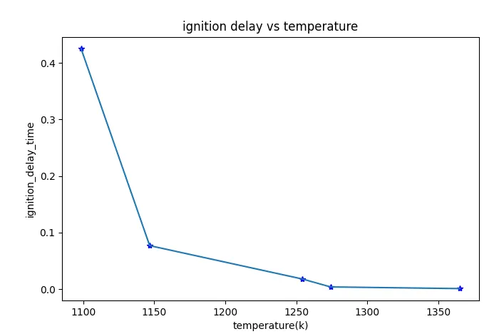

Fig.3 Ignition_delay_time vs temperature

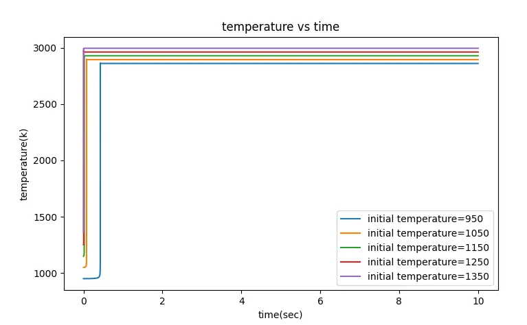
Fig.4 temperature vs time

Case3: the rate of change of molar concentrations of the given elements "H2O, O2, OH" with respect to the time.(when T=1000k,P=5bar)

import cantera as ct
import numpy as np
import matplotlib.pyplot as plt

gas =ct.Solution('gri30.cti')
T=1000
P=5*101325

gas.TPX= T,P,{'CH4':1,'O2':2,'N2':7.52}
r=ct.IdealGasReactor(gas)
sim=ct.ReactorNet([r])
time=0

states=ct.SolutionArray(gas,extra=['tim'])

for n in range(10000):
    time +=1e-3
    sim.advance(time)
    states.append(r.thermo.state,tim=time)
    
plt.subplot(3,1,1)
plt.plot(states.tim,states.X[:,gas.species_index('H2O')])
plt.ylabel('H2O mole fraction')
plt.grid()
plt.subplot(3,1,2)
plt.plot(states.tim,states.X[:,gas.species_index('O2')])
plt.ylabel('O2 mole fraction')
plt.grid()
plt.subplot(3,1,3)
plt.plot(states.tim,states.X[:,gas.species_index('OH')])
plt.ylabel('OH mole fraction')
plt.xlabel('time in sec')
plt.grid()
plt.show()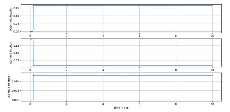

Fig.5 Variation of molar concentration with time(time=1000k)

Case4: The rate of change of molar concentrations of the given elements "H2O, O2, OH" with respect to the time.(when T=500k,P=5bar)

import cantera as ct
import numpy as np
import matplotlib.pyplot as plt

gas =ct.Solution('gri30.cti')
T=500
P=5*101325

gas.TPX= T,P,{'CH4':1,'O2':2,'N2':7.52}
r=ct.IdealGasReactor(gas)
sim=ct.ReactorNet([r])
time=0

states=ct.SolutionArray(gas,extra=['tim'])

for n in range(10000):
    time +=1e-3
    sim.advance(time)
    states.append(r.thermo.state,tim=time)
    
plt.subplot(3,1,1)
plt.plot(states.tim,states.X[:,gas.species_index('H2O')])
plt.ylabel('H2O mole fraction')
plt.grid()
plt.subplot(3,1,2)
plt.plot(states.tim,states.X[:,gas.species_index('O2')])
plt.ylabel('O2 mole fraction')
plt.grid()
plt.subplot(3,1,3)
plt.plot(states.tim,states.X[:,gas.species_index('OH')])
plt.ylabel('OH mole fraction')
plt.xlabel('time in sec')
plt.grid()
plt.show()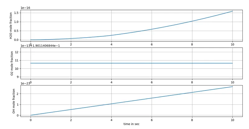

Fig.6 Variation of molar concentration with time(T=500k)