Week 7 - Auto ignition using Cantera

Objective -->>1: To observe the effect of pressure and temperature on the auto-ignition time.

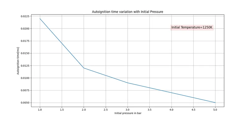
1)plotting the auto ignition time for varying pressure from 1 to 5 atm at constant temperature 1250 K.

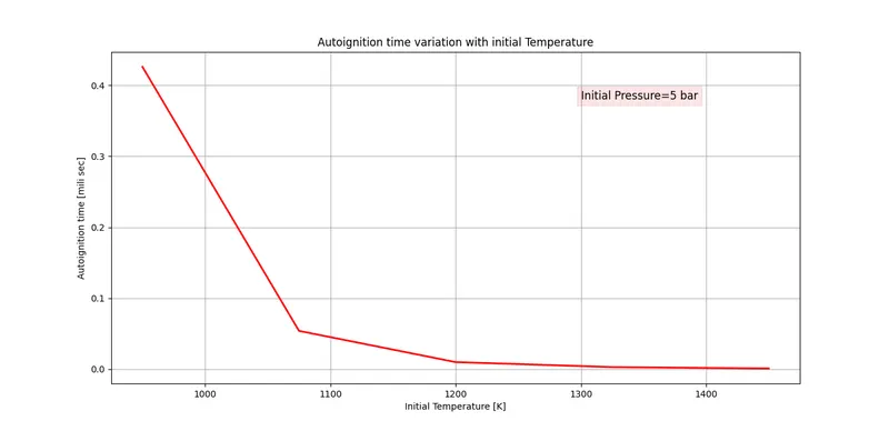
2)plotting the auto ignition time for varying temperatures 950K to 1450K at constant pressure 5atm.

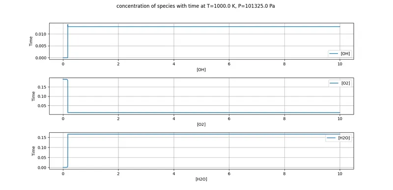
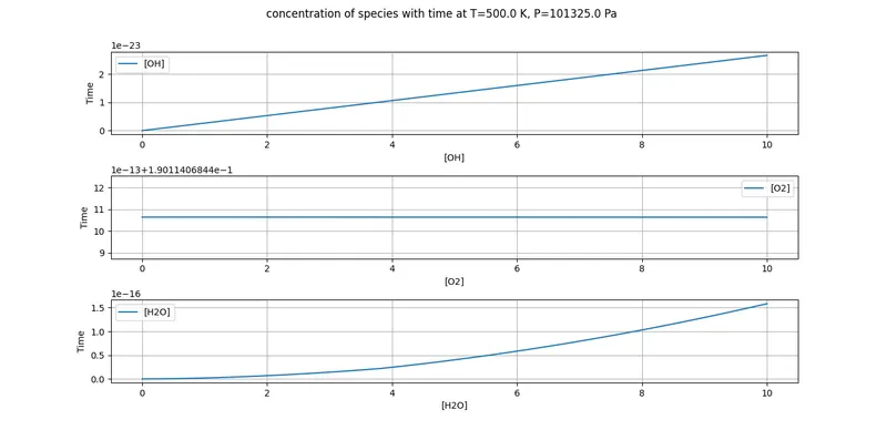
Objective -->>2: To print the rate of change of molar concentration of H2O,O2,OH with respect to time

case 1)Temperature =1000 K and pressure= 5 atm

case 2)Temperature =500 K and pressure= 5 atm

Introduction: For the project, the methane is contained in the cylinder with the stoichiometric composition of fuel and oxidizer.

Autoignition: Autoignition occurs when gas or the mixture of gas ignites spontaneously without any ignition source and that temperature is known as the autoignition temperature, Now that Autoignition temperature is not an intrinsic property of the gas but it depends on pressure, shape, and volume of the vessel, surface activity, etc...

The interval of time between zero to the autoignition time is known as ignition delay.So higher the autoignition time the higher the ignition delay.

Auto_ignition time variation with Temperature:

python code:

# auto ignition time variation with  initial temperature
import matplotlib.pyplot as plt
import numpy as np
import cantera as ct

# creating the array of temperature
T_ini =950
T_end=1450
T=np.linspace(T_ini,T_end,5)

# time for simulation
time=1   # time in seconds
#time for cantera
t_sim_ct=time*1000   # in mili seconds

#creating the solution object gas from solution class
gas = ct.Solution('gri30.yaml')

# for updating the ignition time for each Temperature
t_ig=[]
for i in T:
    
    # defining the temperature and pressure and mole fraction of gas
    gas.TPX=i,5*ct.one_atm,{'CH4':1,'O2':2,'N2':7.52}
    # creating the reactor which will take the argument gas
    r=ct.IdealGasReactor(gas)
    #creating the reactor network which will take reactor as argument
    sim=ct.ReactorNet([r])
    #define the solution states
    states=ct.SolutionArray(gas,extra=['time_in_ms'])
    time=0

    for j in range(t_sim_ct):
        time+=1e-3
        sim.advance(time)
        states.append(r.thermo.state,time_in_ms=time)

    for k in range(t_sim_ct):
        T_error=states.T[k]-i-400
        if (T_error>0):
            t_i=states.time_in_ms[k]
            break
    t_ig.append(t_i)
plt.plot(T,t_ig,color='red',lw=2)
plt.xlabel('Initial Temperature [K]')
plt.ylabel('Autoignition time [mili sec]')
plt.title('Autoignition time variation with initial Temperature')
plt.text(1300,0.38,"Initial Pressure=5 bar",fontsize=12,bbox=dict(facecolor='red',alpha=0.1))
plt.grid()
plt.show()

output

Conclusion

#from the plot we can conclude that the ignition delay is decreasing with increasing initial temperature at constant pressure.

Auto_ignition variation with pressure

python code

# auto ignition variation with pressure 
# constant temperature 1250 K

import numpy as np
import matplotlib.pyplot as plt
import cantera as ct

# creating the gas object 
gas=ct.Solution('gri30.yaml')

# defining the range of P
P=np.linspace(ct.one_atm,5*ct.one_atm,5)

# defininf the simulation time 
t_sim=10   # time in seconds
#cantera uses time in mili seconds so overwriting the t_sim 
t_sim_cantera=t_sim*1000
# defining the empty list for updating them at the eend of iteration

tau=[]

##############################################################
for i in P:
    gas.TPX=1250,i,{'CH4':1,'O2':2,'N2':7.52}

    # creating the reactor r which will take argument gas
    r=ct.IdealGasReactor(gas)
    # creating the Reactornet 
    sim=ct.ReactorNet([r])

    # initial time
    time=0
    states=ct.SolutionArray(gas,extra=['time_in_ms'])
    for j in range(1000):
            time+=1e-3   # its not the dt value it is the value upto which we want to integrate the system ,the value of time step sizze will be decided by cantera itself
            sim.advance(time)   # its going to integrate upto that time
            states.append(r.thermo.state,time_in_ms=time)
     ############
    for k in range(t_sim_cantera):
        T_error=states.T[k]-1250-400
        if T_error>=0:
            T_auto_ig=states.T[k]
            tau_auto_ig=states.time_in_ms[k]
            break
    tau.append(tau_auto_ig)
    #temp_new[:,itr]=states.T
    
plt.xlabel(' Initial pressure in bar')
plt.ylabel('Autoignition time[ms]')
plt.title('Autoignition time variation with Initial Pressure')
 
plt.plot(P/101325,tau)
plt.text(4,0.02,'Initial Temperature=1250K',fontsize=12,bbox=dict(facecolor='red',alpha=0.1))
plt.grid()
plt.show()

output

Conclusion:

# from the plot we can conclude that by increasing initial pressure ignition delay is decreasing with constant initial temperature.

variation of concentration of the species with time

python code

# Rate of change of molar concentration of H2O,O2,OH with respect to time
 
import cantera as ct
import numpy as np
import matplotlib.pyplot as plt

gas=ct.Solution('gri30.yaml')
T=500
P=ct.one_atm
gas.TPX=1000,5*ct.one_atm,{'CH4':1,'O2':2,'N2':7.52}
r=ct.IdealGasReactor(gas)
sim=ct.ReactorNet([r])
states=ct.SolutionArray(gas,extra='time_in_ms')
time=0
t=[]

for i in range(10000):
    time+=1e-3
    sim.advance(time)
    states.append(r.thermo.state,time_in_ms=time)
    t.append(time)
    states.X
M_H2O=states.X[:,gas.species_index('H2O')]
M_O2=states.X[:,gas.species_index('O2')]
M_OH=states.X[:,gas.species_index('OH')]

fig, axes=plt.subplots(3,figsize=(8,8),gridspec_kw={'width_ratios':[3],'height_ratios':[3,3,3],'wspace':0.4,'hspace':0.5})

ax1=axes[0]
ax1.plot(t,M_OH,label='[OH]')
ax1.set_xlabel('[OH]')
ax1.set_ylabel('Time')
ax1.legend()
ax1.grid()

ax2=axes[1]
ax2.plot(t,M_O2,label='[O2]')
ax2.set_xlabel('[O2]')
ax2.set_ylabel('Time')
ax2.legend()
ax2.grid()

ax3=axes[2]
ax3.plot(t,M_H2O,label='[H2O]')
ax3.set_xlabel('[H2O]')
ax3.set_ylabel('Time')
ax3.legend()
ax3.grid()

plt.suptitle("concentration of species with time at T=%0.1f K" %T + ", P=%0.1f Pa " %P)
plt.show()

output

conclusion:

from the plot at 500 K we can say that ignition is not yet started because the concentration of the products [H2O],[OH] is at 0

and at the temperature 1000K the [H2O] and[OH] is increased up to certain value which means combustion process has occurred that means the autoignition temperature of CH4 is in the range of 500K to 1000K.