Week 7 - Auto ignition using Cantera

Auto ignition using Cantera

PART I

Aim:

To simulate the Auto Ignition Time for Methane-air mixture under the following conditions, (simulation time = 10 secs).

To plot the variation of Auto Ignition time of Methane with a constant temperature of 1250K and pressure varying from 1 to 5 atm.

To plot the variation of Auto Ignition time of Methane with a constant pressure of 5 atm and temperature varying from 950K to 1450K.

Description:

Auto Ignition time:

When air-fuel mixture present at room temperature, any pressure and composition is heated slowly, at some minimum temperature for the given pressure and composition the mixture will ignite automatically. This temperature is called as Auto ignition Temperature. This is not just a property of the fuel, but also depends on pressure and composition.

When we take a closer look into the system, when the system is heated to a temperature above Auto ignition temperature, the combustion process will not takes place instantaneously. However the delay time for combustion is very small (order of milliseconds). This time delay for combustion is called Auto Ignition Time or Ignition delay. This Auto Ignition Temperature depends on Temperature, pressure and composition.

The need for estimating this time is important because, in all the combustion devices in flow of reactants and out flow of products takes place at very high speeds. So we need to make sure that the combustion time scales are much smaller than the flow time scales. For example in case of diesel engines, the time for power stroke must be much larger than the ignition delay.

This is also used for validating the results obtained from chemical kinetics mechanisms with the experimental data. This gives us the confidence that, our mechanism is simulating the actual combustion process accurately.

For calculating the Auto Ignition time, we look for the time it takes for the system to reach a temperature of initial temperature + 400K.

Code:

Function code for calculating properties at each intermediate time step.

""" 
This fucntion calculates the properties of system at each time step
and return the object containg properties
"""
def cv_combust(T,P,species_dict):

	import sys
	import numpy as np
	import matplotlib.pyplot as plt
	import cantera as ct
	gas  = ct.Solution('gri30.xml')
	gas.TPX = T,P,species_dict

	r = ct.IdealGasReactor(gas)

	sim = ct.ReactorNet([r])
	time = 0.0
	states = ct.SolutionArray(gas,extra = ['time_in_ms','t'])

	for n in range (10000):
		time +=1e-3
		sim.advance(time)
		states.append(r.thermo.state,time_in_ms = time*1e3,t = time)



	return states

Code for plotting the required graph:

""" 
This fucntion calculates the properties of system at each time step
and return the object containg properties
"""
def cv_combust(T,P,species_dict):

	import sys
	import numpy as np
	import matplotlib.pyplot as plt
	import cantera as ct
	gas  = ct.Solution('gri30.xml')
	gas.TPX = T,P,species_dict

	r = ct.IdealGasReactor(gas)

	sim = ct.ReactorNet([r])
	time = 0.0
	states = ct.SolutionArray(gas,extra = ['time_in_ms','t'])

	for n in range (10000):
		time +=1e-3
		sim.advance(time)
		states.append(r.thermo.state,time_in_ms = time*1e3,t = time)



	return states



"""
This code calculates the auto ignition temperature
"""
import matplotlib.pyplot as plt
import numpy as np
import math

# loop for accounting variation of pressure from 1 to 5 atm
ignition_delay = []
pressure = []
for i in range (7):
	T = 1250
	P = (5-((6-i)*4)/6)
	# considering stoichiometric composition
	y = cv_combust(T,P*101325,{'CH4':1,'O2' : 2,'N2' : 7.52})
	# calculating ignition delay
	j = 0
	
	while (y.T[j] < T+400):
			j = j+1

	ignition_delay.append(j)
	pressure.append(P)

plt.plot(pressure,ignition_delay,'b-*')
plt.xlabel("pressure (atm)")
plt.ylabel("Auto Ignition Delay")
plt.title("Ignition delay w.r.t initial pressure")
plt.grid('on')
plt.show()


# loop for accounting variation of temperature from  950 to 1450K
ignition_delay = []
temperature = []
for i in range (10):
	P = 5*101325
	T = (1450-((9-i)*500)/9)
	# considering stoichiometric composition
	y = cv_combust(T,P,{'CH4':1,'O2' : 2,'N2' : 7.52})
	# calculating ignition delay
	j = 0
	
	while (y.T[j] < T+400):
			j = j+1

	ignition_delay.append(j)
	temperature.append(T)

plt.plot(temperature,ignition_delay,'b-*')
plt.xlabel("temperature (K)")
plt.ylabel("Auto Ignition Delay")
plt.title("Ignition delay w.r.t initial temperature")
plt.grid('on')
plt.show()

Results:

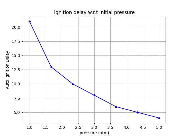
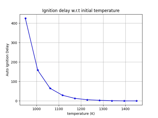
Comments:

Auto ignition delay temperature is decreasing with increase in pressure and temperature.

For most of the reactions Auto ignition time decreases with increase in temperature, because of increase in collision frequency which reflects in reaction rate.

Effect of pressure depends on the reaction in discussion.

PART II

Aim:

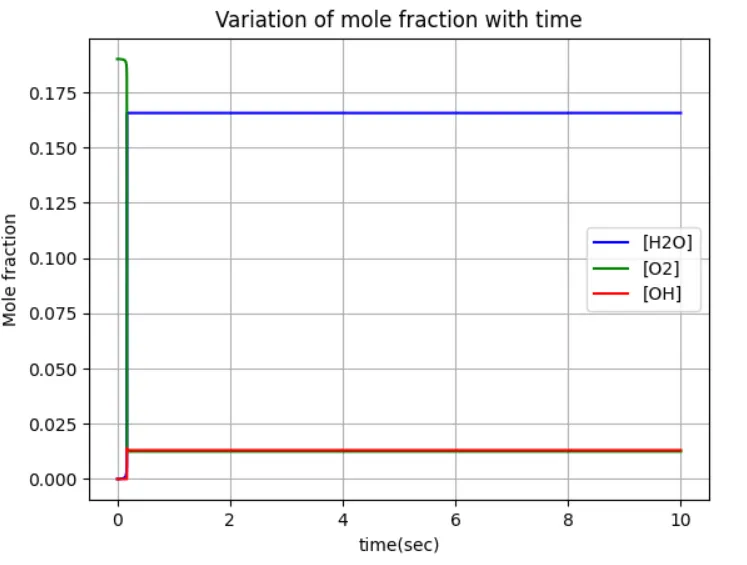
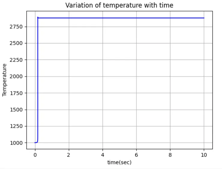
To observe and print the rate of change of molar concentrations of the elements "H2O, O2, OH" with respect to the time, (simulation time = 10 secs)

When Temperature is 1000K and Temperature is 500K and pressure 5 bar for both cases.

Code:

"""
This code calculates the composition of species
"""
import matplotlib.pyplot as plt
import numpy as np
import math
import cantera as ct

# calculating molar concentrations at 5 bar and 1000K

T = 1000

P = 5*101325
# considering stoichiometric composition
gas  = ct.Solution('gri30.xml')
gas.TPX = T,P,{'CH4':1,'O2' : 2,'N2' : 7.52}

r = ct.IdealGasReactor(gas)

sim = ct.ReactorNet([r])
time = 0.0
states = ct.SolutionArray(gas,extra = ['time_in_ms','t'])

for n in range (10000):
	time +=1e-3
	sim.advance(time)
	states.append(r.thermo.state,time_in_ms = time*1e3,t = time)
plt.figure()
plt.plot(states.t,states.X[:,gas.species_index('H2O')],'b-')
plt.plot(states.t,states.X[:,gas.species_index('O2')],'g-')
plt.plot(states.t,states.X[:,gas.species_index('OH')],'r-')
plt.xlabel("time(sec)")
plt.ylabel("Mole fraction")
plt.title("Variation of mole fraction with time")
plt.legend(['[H2O]','[O2]','[OH]'])
plt.grid('on')
plt.show()

plt.figure()
plt.plot(states.t,states.T,'b-')
plt.xlabel("time(sec)")
plt.ylabel("Temperature")
plt.title("Variation of temperature with time")
plt.grid('on')
plt.show()

Plots:

Temperature = 500K and Pressure = 5 atm

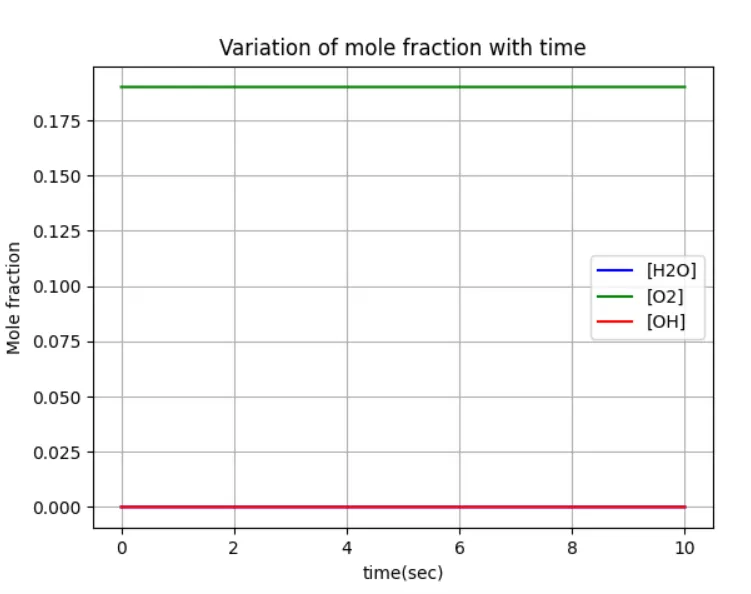
Note:mole fraction of both `H_2O` and OH are zero, as reaction is not taking place.

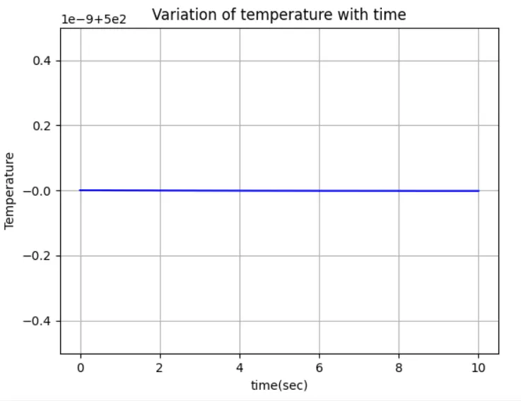
Temperature = 1000K and Pressure = 5 atm

Comments:

At 500K reaction is not taking place, as the temperature is less than auto ignition temperature.

At 1000K reaction takes place.

Auto ignition temperature for methane and air stoichiometric mixture is arround 800K.