Multivariate Newton Rhapson Solver

In this article/project, we will write a python script for solving a set of non-linear coupled Ordinary Differential Equations.

Consider the below set of equations.

Properties of the above equations

• Non-linear - There are terms of second order.
• ODE - Differentials are Ordinary and not partial or substantial.
• Coupled - The variables are spread across different equations.

Let us modify one of the above equations a bit

`dy_1/dt=-0.04y_1+10^4y_2y_3`

Apply backward differencing (The differencing method can vary based on approach)

`((dy_1)^n-(dy_1)^(n-1))/dt=-0.04y_1+10^4y_2y_3`

There are two approaches that we can take to solve these equations.

1. Explicit: In this case, all our R.H.S values will be from the previous timestep. This will make the script easy to write. The problem with the explicit approach is that it is susceptible to time step size and requires it to be very small. Thus, making it computationally expensive.

2. Implicit: This approach uses values from the current timestep in RHS to resolve LHS. This approach is harder to code. But this solves the problem of the timestep. It can use substantially larger timesteps when compared with the Explicit approach.

`((y_1)^n-(y_1)^(n-1))/dt=-0.04(y_1)^n+10^4(y_2)^n(y_3)^n`

`[-0.04(y_1)^n+10^4(y_2)^n(y_3)^n]dt+(y_1)^(n-1)-(y_1)^n=0`

Consider the above equation as f1. Similarly derive the other equations - f2 and f3.

`f1=[-0.04(y_1)^n+10^4(y_2)^n(y_3)^n]dt+(y_1)^(n-1)-(y_1)^n=0`

Newton Raphson Method

Univariate Newton-Raphson Method

`y^(n+1)=y^n-alphaf(y^n)/f^'(y^n)`

where alpha is the relaxation factor.

Refer to the below video to understand the Math of the univariate Newton-Raphson Method.

Multivariate Newton Raphson Method

`y^(n+1)=y^n-alphaJ^-1F`

where J is the Jacobian matrix.

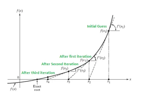
Mathematical equations can be hard to understand, so here is a visual understanding of the Newton-Raphson method.

Jacobian

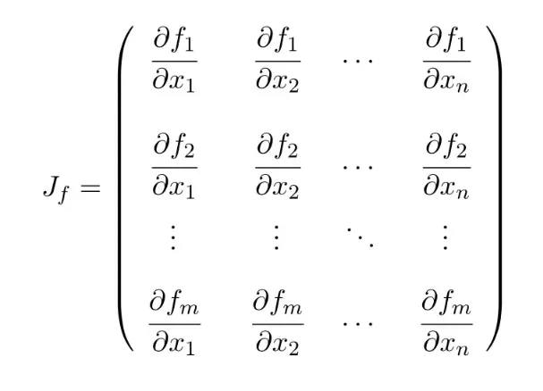
Jacobian Matrix is given by the following expression. Here, f1,f2...fm are m functions dependent on x1,x2....xn variables.

Jacobian Matrix gives partial derivatives of all the functions w.r.t all the variables.

Code

Import necessary libraries

import math
import numpy as np
from numpy import linalg
import matplotlib.pyplot as plt

Define functions f1,f2,f3

def f1(y,yOld1,dt): 
    return (-0.04*y[0]+1e4*y[1]*y[2])*dt+yOld1-y[0]

def f2(y,yOld2,dt):
    return (0.04*y[0]-1e4*y[1]*y[2]-3*1e7*pow(y[1],2))*dt+yOld2-y[1]

def f3(y,yOld3,dt):
    return (3*1e7*pow(y[1],2))*dt+yOld3-y[2]

Define function Jacobian

For the first term of the Jacobian Matrix, in python terms J(0,0)

`(df_1)/dy_1=(f_1(y_1+dy,y_2,y_3)-f_1(y_1,y_2,y_3))/dt`

All the other terms can be found in a similar way.

def jacobian(yNew,yOld,dt):

    dy=1e-10

    Y1=[yNew[0]+dy,yNew[1],yNew[2]]
    Y2=[yNew[0],yNew[1]+dy,yNew[2]]
    Y3=[yNew[0],yNew[1],yNew[2]+dy] 

    J=np.ones([3,3])

    yOld1=yOld[0]
    
    yOld2=yOld[1]
    yOld3=yOld[2]

    J[0,0] = (f1(Y1,yOld1,dt) - f1(yNew,yOld1,dt))/dy
    J[0,1] = (f1(Y2,yOld2,dt) - f1(yNew,yOld2,dt))/dy
    J[0,2] = (f1(Y3,yOld3,dt) - f1(yNew,yOld3,dt))/dy

    J[1,0] = (f2(Y1,yOld1,dt) - f2(yNew,yOld1,dt))/dy
    J[1,1] = (f2(Y2,yOld2,dt) - f2(yNew,yOld2,dt))/dy
    J[1,2] = (f2(Y3,yOld3,dt) - f2(yNew,yOld3,dt))/dy

    J[2,0] = (f3(Y1,yOld1,dt) - f3(yNew,yOld1,dt))/dy
    J[2,1] = (f3(Y2,yOld2,dt) - f3(yNew,yOld2,dt))/dy
    J[2,2] = (f3(Y3,yOld3,dt) - f3(yNew,yOld3,dt))/dy

    return J 

Defining Constants and Array used in the script

yOld=np.zeros([3,1])
yOld[0]=1

yNew=np.zeros([3,1])

yGuess=np.zeros([3,1])
yGuess[0]=1

dt=0.1      #Time step size
t=600       #Total time = 10*60 sec

error=9e9
tol=1e-6
alpha=1

Time=np.arange(0,600,dt)
Y1 = np.zeros((3, int(600/dt)))  #For plotting

For loop

for i in range(0,int(t/dt)):

    F=np.copy(yNew)
    yGuess=np.copy(yOld)
    
    while error>tol:
        
        J=jacobian(yNew,yOld,dt) 

        F[0]=f1(yGuess,yOld[0],dt)
        F[1]=f2(yGuess,yOld[1],dt)
        F[2]=f3(yGuess,yOld[2],dt)

        yNew=yGuess-alpha*np.matmul(linalg.inv(J),F)
        
        ABS=abs(yNew-yGuess)
        error=np.max(ABS)
        yGuess=yNew

    yOld=yNew
    Y1[:, i] = yNew[:,0]
    error=1e9

Plotting

plt.plot(Time,Y1[0, :], label = 'y1')
plt.plot(Time,Y1[1,:], label = 'y2')
plt.plot(Time,Y1[2, :], label = 'y3')
plt.title('Multi-variate Newton Raphson Solver for dt = ' +str(dt))
plt.xlabel('Time (secs)')
plt.ylabel('y_i')
plt.legend()
plt.grid()
plt.show()

Result

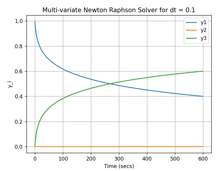
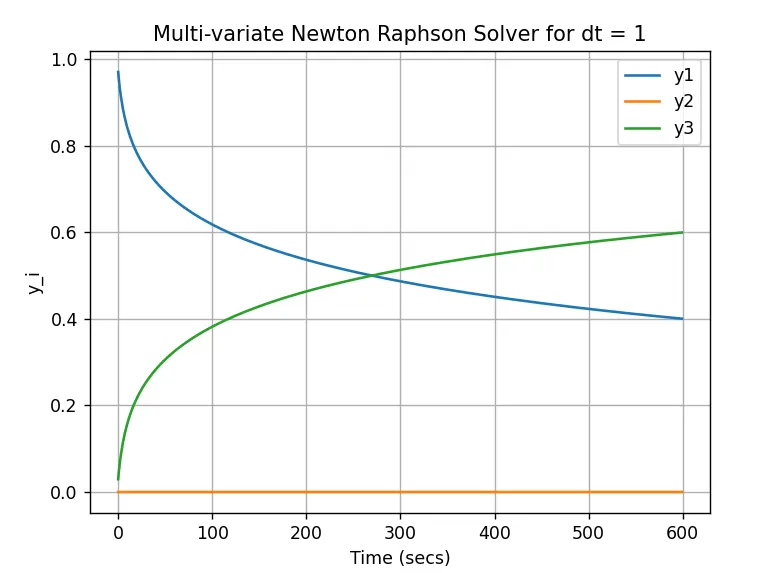
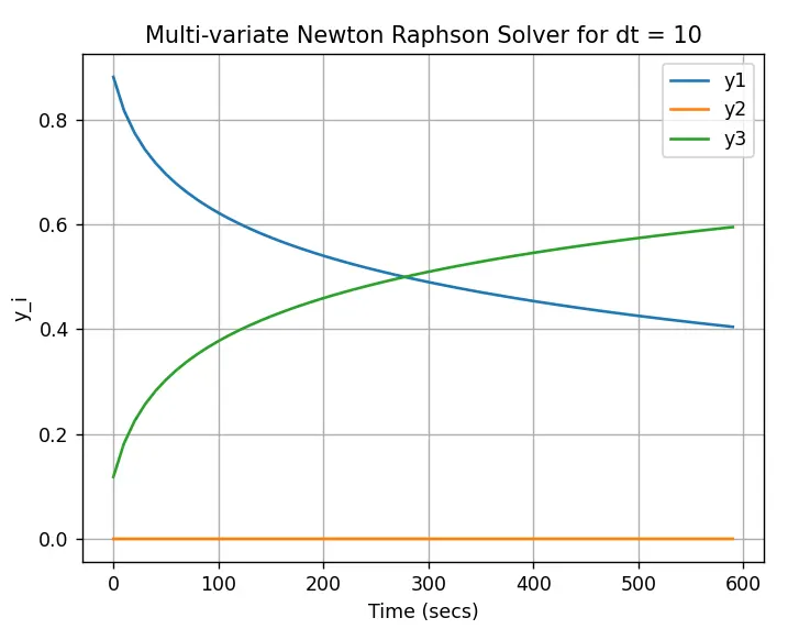
From the above plots, it is observed that as the time step is increased, there is not much change in the pattern of the plots. This is because the Implicit approach allows us to use higher-time steps while giving accurate results.

It is also noteworthy that, as time steps are increased, the extreme values i.e. values of y1,y2, and y3 at initial and final time steps tend to deviate from the original values.