Week 6: Conjugate Heat Transfer Simulation
Aim
To conduct a transient Conjugate Heat Transfer simulation on the given pipe geometry with specified heat flux and verify the outlet temperature using various mesh sizes. Further, change the supercycle state interval to observe its effect on the total simulation time.
Introduction
Conjugate Heat Transfer (CHT) comprises heat transfer in solids, dominated by conduction, and heat transfer in fluids, dominated by convection. The processes are divided into two subdomains and are calculated separately using their respective governing equations. Conditions at the interface of the two are then used to determine the distribution of the temperature/heat flux. Conjugate heat transfer analyses are quite often used in HVAC systems, heat sinks, engine cooling, etc.
An important challenge to overcome in conjugate heat transfer simulations is the disparity in time scales between the heat transfer in fluids and solids. Heat transfer in solids is generally much slower than that of in fluids and this increases the computational budget for simulations with long time periods. One method which Converge uses to solve this problem is by using Super-cycling. Super-cycling involves freezing the fluid solver periodically when solving for the heat transfer in solids using the time-averaged fluid quantities in the interval. This method drastically reduces the computational cost and quickens the overall simulation.
Method
Domain and Mesh
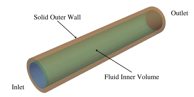
The geometry of the pipe channel was provided and can be seen in the schematics below. The length of the pipe is 0.2m and has an internal diameter of 0.03m and an outer diameter of 0.04m.
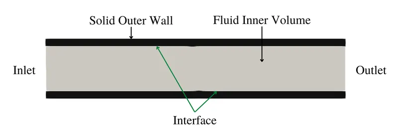
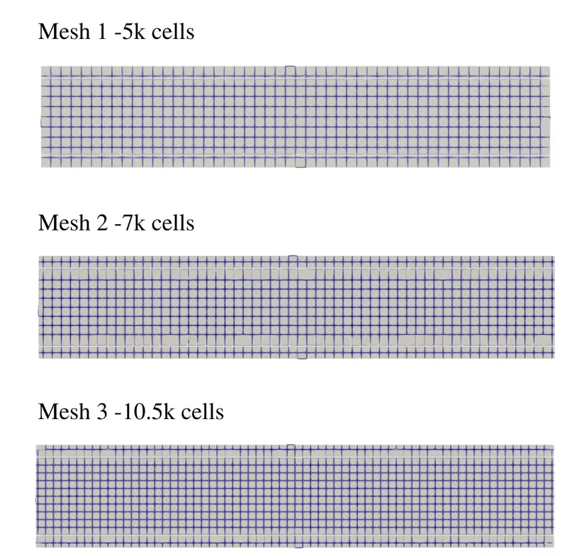
An unstructured cartesian grid was generated over the geometry. A total of three meshes were generated with varying element sizes of 4mm, 3.5mm, and 3mm respectively. The results of the mesh generation can be seen in the image below.
CFD Setup
All Simulations were conducted using Converge v3.0. The fluid used in the domain was air with default properties. To ensure flow inlet Reynolds number of 7000, the velocity at the inlet was computed as:
`V = Re*mu/(rhoD)`
`V = 7000* (1.81e-5)/(1.225*0.03)`
V = 3.45 m/s
The pressure outlet was set to 1 atm. The solid used in the domain was Aluminium with default properties. The outer walls of the pipe were provided with a heat flux of -10000`Wm^-2`. The forward side of the interface was set to the fluid region with a wall treatment of law of the wall. The reverse side of the interface was set to the solid region with a specified value temperature boundary condition coupled to the fluid volume.
The transient density-based PISO solver was used for the spatial discretization of the flow parameters. Turbulence in the flow was estimated using the two-equation standard K-Epsilon Model. Momentum, density, turbulence, energy, and species were estimated using the SOR scheme while pressure was estimated using the converge bicgstab scheme. Super-cycling was enabled for the simulation with a monitor point on the solid near the outlet. The time interval for the super-cycling stage was initially set to 0.05s and then varied to 0.03, 0.02, and 0.01s.
The variable time stepping method was used for the simulation with minimum and maximum time step sizes of 1e-7s and 1s respectively. The max CFL number of the system was limited to 1. The simulation was conducted for a total time of 0.5s.
Results
The image below shows the temporal variations of the average temperature at the outlet for the various meshes. It can be seen that all the meshes converge to a particular value upon reaching a steady state.
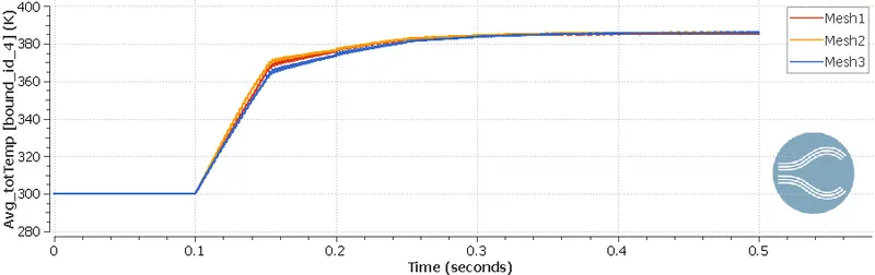
Since all meshes predict a similar temperature at the outlet, Mesh 2 was chosen as the final mesh to conduct further simulations as it is more refined than Mesh 1 and computationally cheaper than Mesh 3.
The image below shows the yplus distribution for the various meshes.
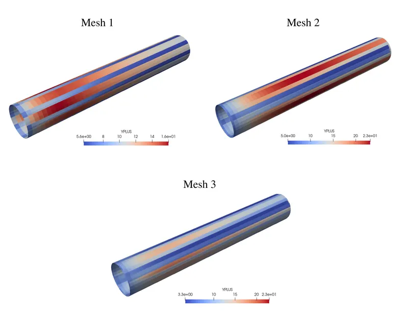
From the images, it can be seen that the yplus for all the mesh cases is consistently within the buffer region. To ensure the first cell of the mesh is in the log law region for ideal working of wall functions, the mesh near the walls needs to be coarsened.
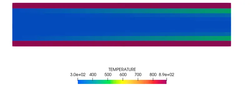
The image below shows the temperature distribution at the mid-plane at t=0.05s.
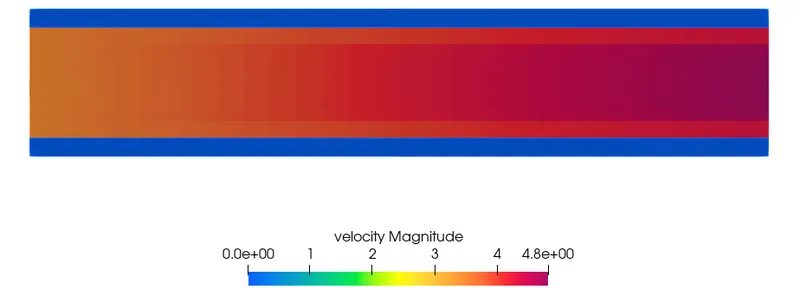
The image below shows the velocity distribution at the mid-plane at t=0.05s.
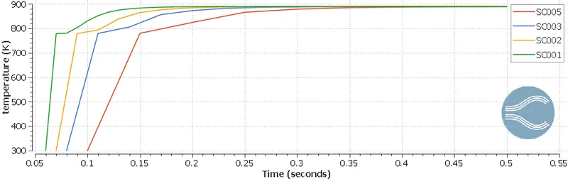
The image below shows the temporal variation of temperature for the various super-cycling intervals (0.01s, 0.02s, 0.03s, 0.05s).
| Case | Super-Cycling Interval [s] | Simulation Run time [s] |
| 1 | 0.01 | 5522 |
| 2 | 0.02 | 5501 |
| 3 | 0.03 | 5460 |
| 4 | 0.05 | 2884 |
From the above results, it can be seen that increasing the super-cycling interval reduces the simulation run time significantly. However, the simulation does take longer to achieve a steady state compared to smaller super-cycling intervals and may lead to solution instabilities. Therefore, choosing an optimum super-cycling interval is essential to reduce the computational cost of simulation and increase solution stability.
Drive link to the animation:
https://drive.google.com/file/d/1D2TS2kpALJF_XtpwrGOt4M-nYz70U3OV/view?usp=sharing
Conclusion
The transient conjugate heat transfer simulation on the given pipe geometry was conducted using converge. Simulations were conducted for varying mesh sizes to verify the convergence of the average temperature at the outlet. The Super-cycling time intervals were varied for simulations and were seen to significantly alter the simulation run time. Increasing the super-cycling time intervals showed a decrease in simulation run time with an increase in the time taken to reach a steady state and vice versa. Therefore, an optimum super-cycling interval was deemed essential to reduce the computational cost of simulation and maintain solution stability.