Week 6: Conjugate Heat Transfer Simulation

AIM: Conjugate heat transfer simulation using CONVERGE in a pipe flow.

OBJECTIVE:

• To run grid dependence test on 3 grid size.
• effect of supercycle stage interval i,e, 0.01,0.02,and 0.03.
• To show temperature converges to a particular value.

INTRODUCTION:

As we know 3D Transient heat conduction equation:

`rho*c_p*(delT)/(delt)=grad.(k*gradT)+S_h`

The L.H.S denotes the change of temp. with respect to time and the first term in R.H.S is heat flux due to conduction.

• CONVERGE solves the fluid heat transfer using the energy equation.
• It solves the solid heat transfer using the solid heat equation.

CHT modelling set up

• First of all we have to define fluid and solid materials and their physical properties.
• Configure the fluid and solid region.Assign regions to stream.
• Using appropriate boundary conditions for the boundaries that separates different regions.
• After that selecting time control method ( transient, steady-state, super-cycle).

• Basically ,CHT analysis is done to take temperature distributions and take it to finite element analysis solver to perform thermal analysis.
• As we know the hot spots causes thermal stresses and if they are cyclic in nature(keep on ocuring) leads to failure due to fatigue.
• It is important for thermal and design engineers to know thermal load profile in order to quantify the life of components.

CASE SET UP

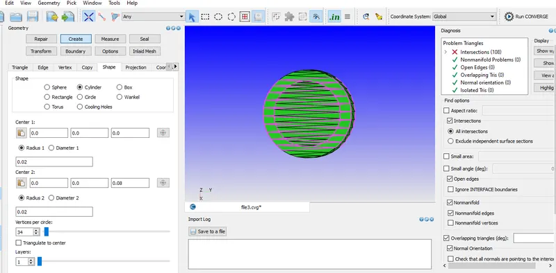
Fig.1 intersection ( overlapping triangles)

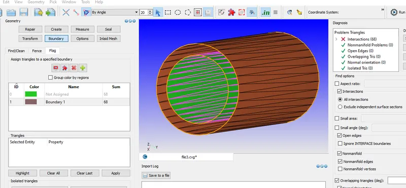
Fig.2 creating thickness for the pipe

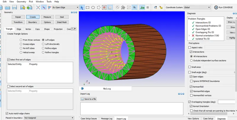
Fig.3

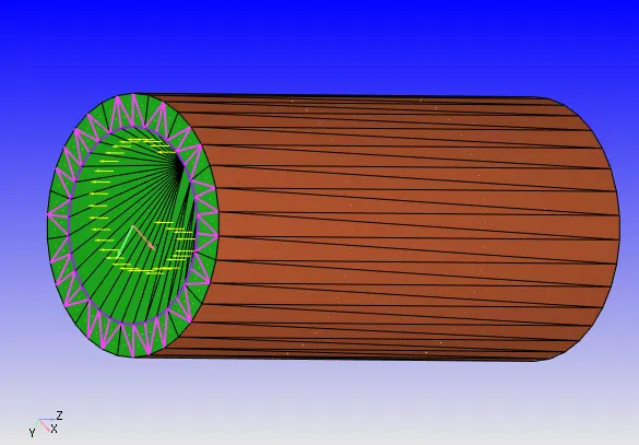
Fig.4

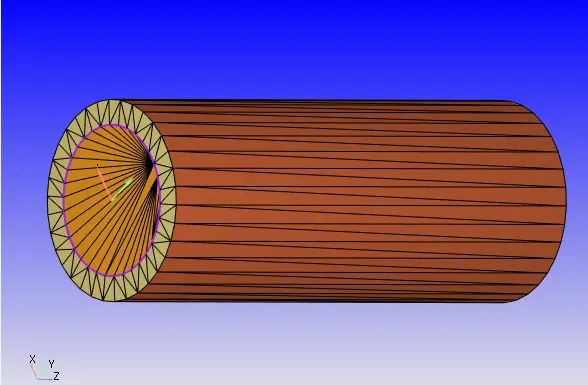
Fig.5 Pipe geometry

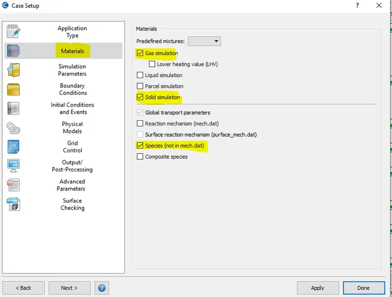
Fig.6 material selection case set up

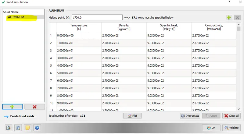
Fig.7 solid material properties

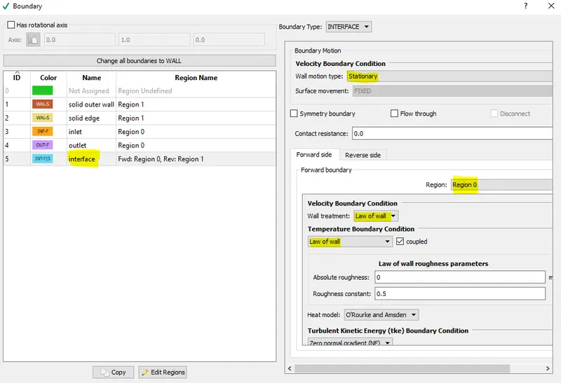
Fig.8 Boundary set up for interface boundary (forward side)

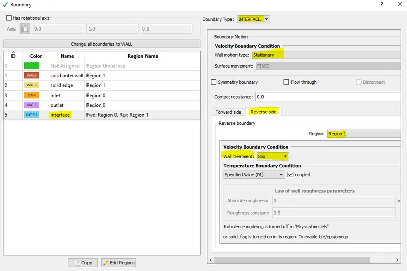
Fig.9 Boundary set up for interface boundary (reverse side)

• An interface boundary indicates two different materials or phases.
• We must define boundary conditions for the forward and reverse boundary of each interface.
• The boundary facing the directon of normal vectors is the forward boundary.
• The boundary facing the opposite direction of the normal vectors is the reverse boundary.

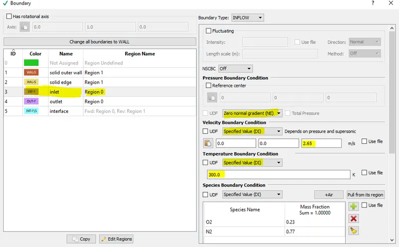
Fig.10 Inlet boundary condition

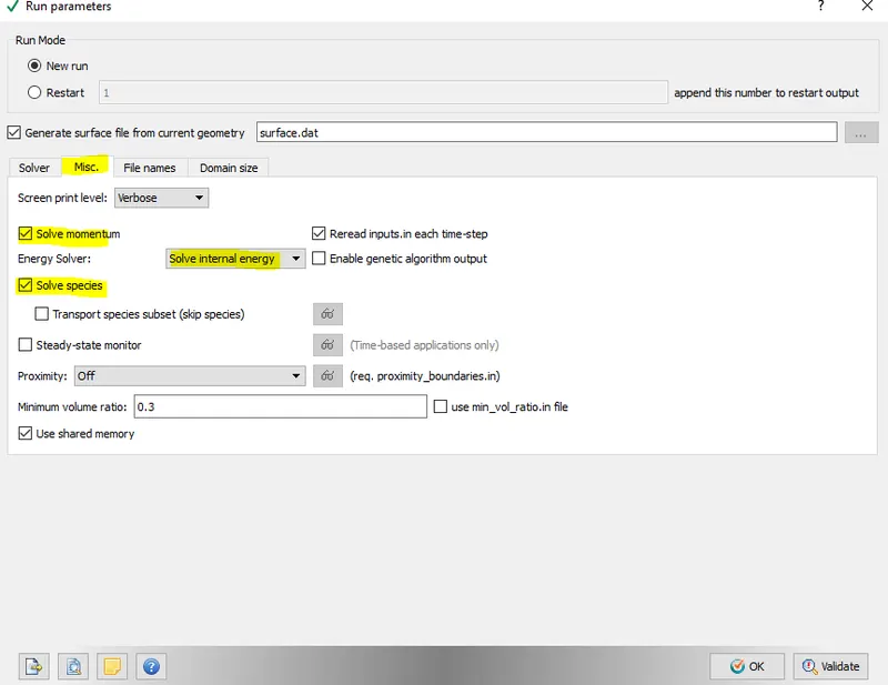
Fig.11 run parameter case set up

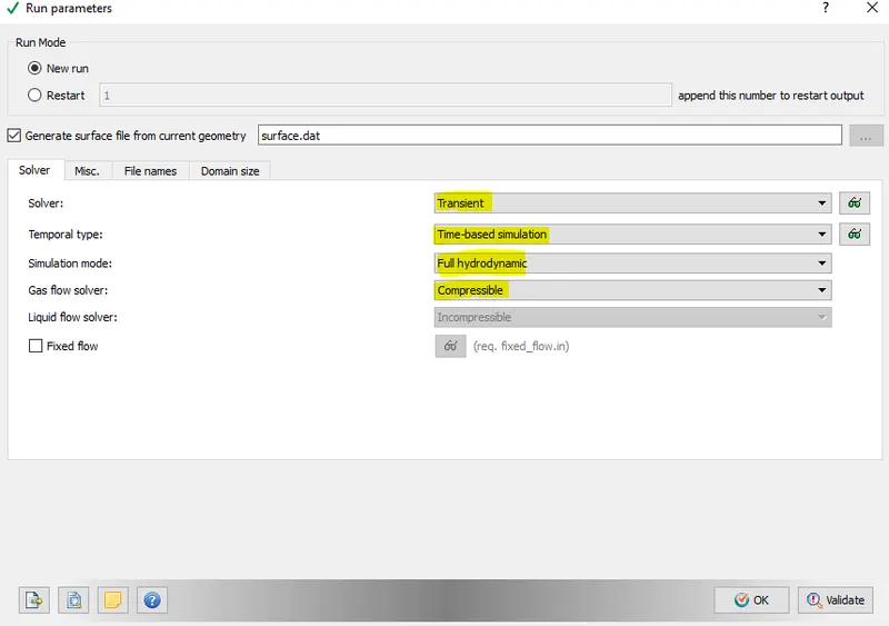
Fig.12

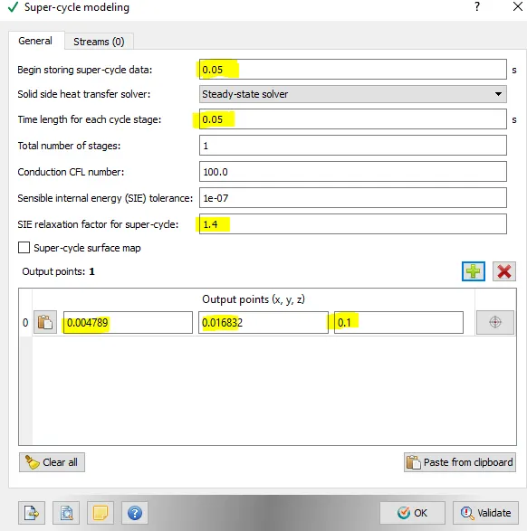
Fig.13 super cycling with cycle interval 0.05

• super-cycling: This is the transient solver which solves the fluid and solid together. For solid itis solving the energy equation(3D heat transient heat conduction equation) and for liquids it is N.s equations.
• It stores the instantaneous HTCs and temperature on the interface during the process.
• After that it freezes the fluid solver.
• Then time averages the HTCs and temp. and apply them as boundary conditions at the interface.
• Solves the solid temperature until it reaches the steady state condition.
• After that updating the solid temp. field and unfreezes the fluid solver.
• repeating unti the solid temperature converges

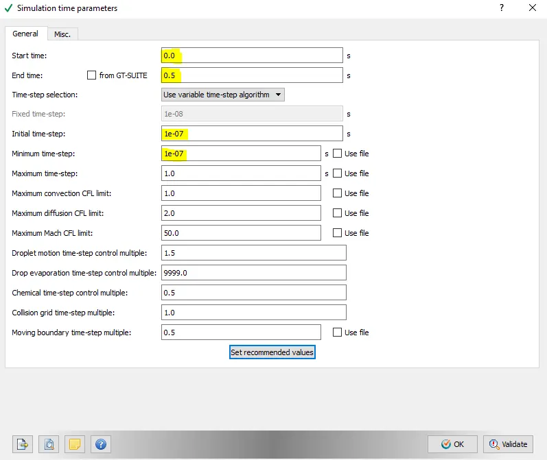
Fig.14 simulation time parameter

• simulation time parameter: start time : 0

end time :0.5 sce

initial time step : 1e-7 sec

minimum time step: 1e-7 sec

maximum time step: 1sec

RESULTS:

PLOTS

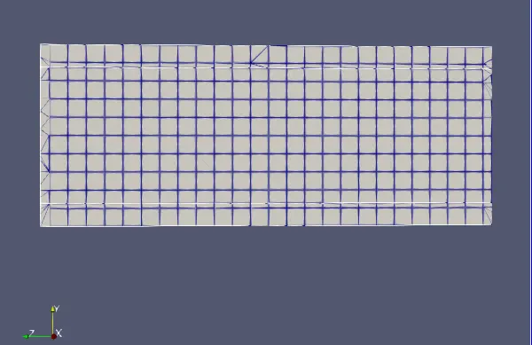
Fig.15 mesh grid 4mm

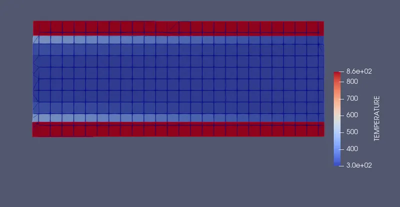
Fig.16 Temperature contour

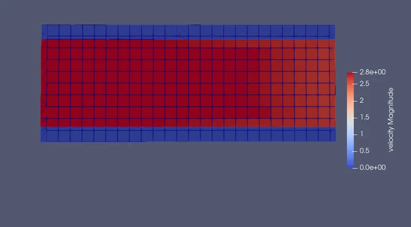
Fig.17 velocity contour

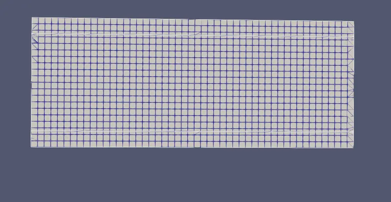
Fig.18 mesh grid 2mm

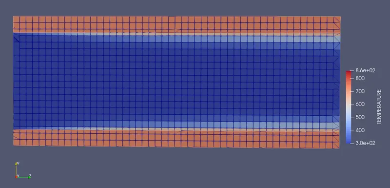
Fig.19 Temperature contour (2mm mesh size)

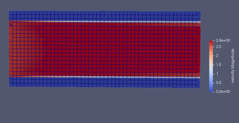
Fig.20 velocity contour( 2mm mesh size)

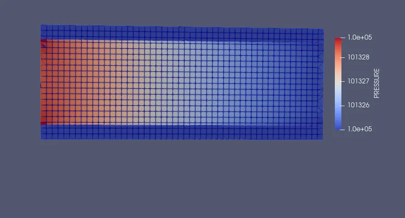
Fig.21 Pressure contour( 2mm mesh size)

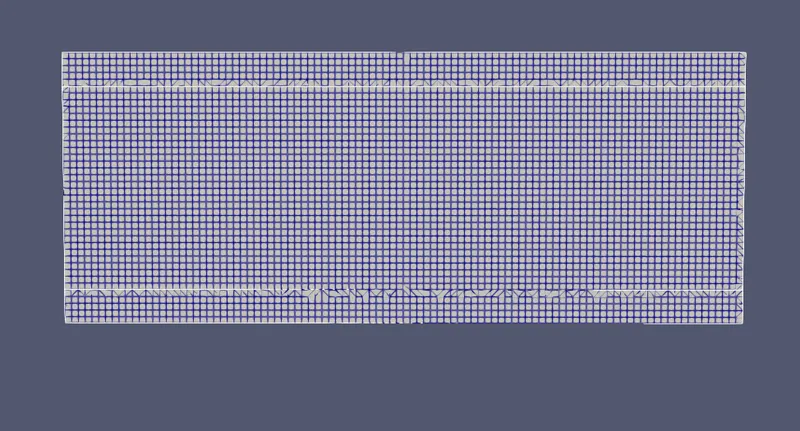
Fig.22 grid size 1mm

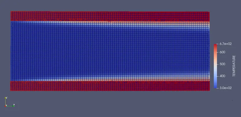
Fig.23 Temperature contour (1mm mesh size)

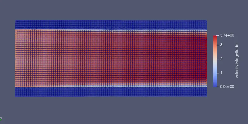
Fig.24 Velocity contour( 1mm mesh size)

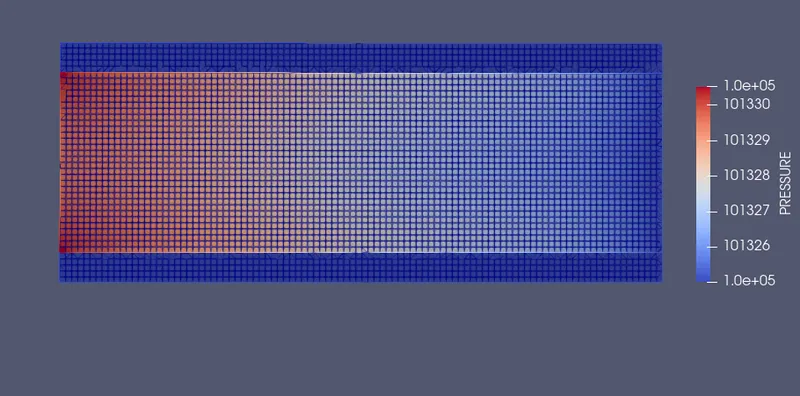
Fig.25 Pressure contour (1mm mesh size)

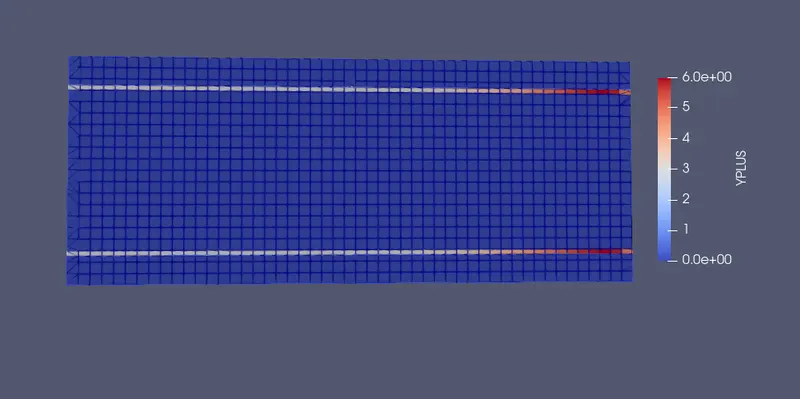
Fig.26 Y-plus for 2mm mesh size

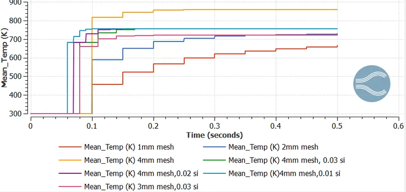
Fig.27 Mean temperature

• For the same mesh size ,if we decrease the super-cycle stage interval ,the solid temperature attains to final steady state at a earlier stage than others.
• For same super-cycle stage interval , if we decreses the mesh size for attaining the steady state temperature requires more cycle.

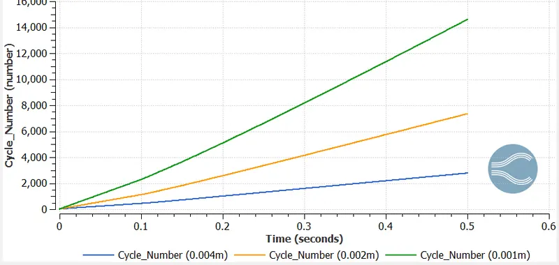
Fig.28 cycle number vs time

• As the mesh size decreases the number of grid points increases so that cycle number also increases for convergence to happen.

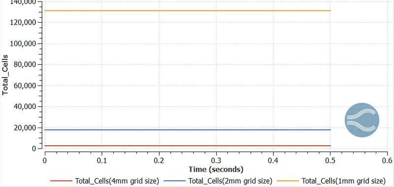
Fig.29 Total cell for different grid size

• Temperature animation ,mesh size 4mm

https://youtu.be/gRI9XoC85w4

• Temperature animation ,mesh size 2mm

https://youtu.be/qXM0ee5TLhU

• Temperature animation ,mesh size 1mm

https://youtu.be/zh_MmSixpww

CONCLUSION:

• CHT analysis is studied by taking solid material as aluminium and fluid as air.
• The simulation is carried out by creating a geometry of cylinder in CONVERGE studio. Three differnt mesh sizes are taken i.e, 4mm,2mm and 1mm grid size.
• For super-cycling stage interval,we varied to 0.03 and 0.01 from 0.05 respectively.
• Here the k-epsilon turbulence model is used.
• The steady state temperature attainment is seen faster as we decreases the super-cycle stage interval.