Week 6 - CHT Analysis on a Graphics card
Aim :-
Perform a steady-state conjugate heat transfer analysis on a model of a graphics card. You can use appropriate materials of your choice for the simulation. Make sure to properly define the correct solid and fluid zones.
Run the simulation for the best possible mesh with a combination of coarse and refined mesh in different regions. Explain the reason for choosing the particular mesh settings.
Expected results:
- Run the simulation by varying the velocity from 1m/sec to 5m/sec for at least 3 velocities and discuss the results.
- Run the simulation by changing the flow pattern and discuss the results.
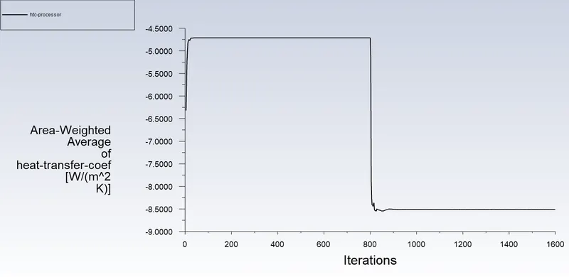
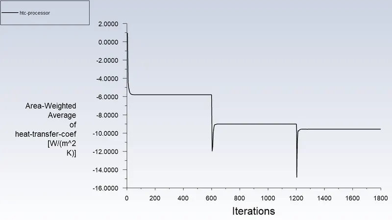
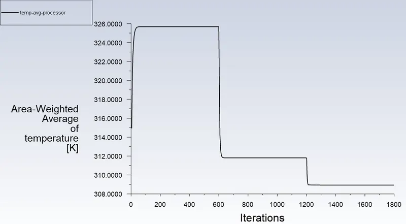
- Find out the maximum temperature and heat transfer coefficient obtained by the processor.
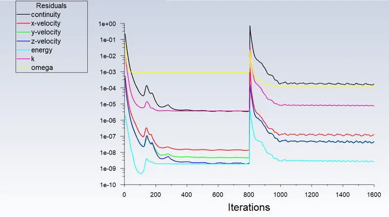
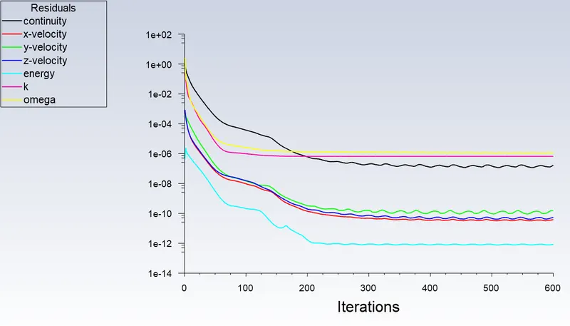
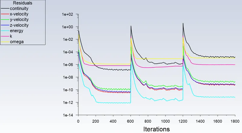
- Prove that the simulation has achieved convergence with appropriate images and plots.
- Identify potential hotspots on the model.
Introducion :-
Procedure :-
- Open workbech with the fluen module and import the geometry in the spaceclaim.
- Now we can see that there is already an enclosure build so no need to build an enclosure
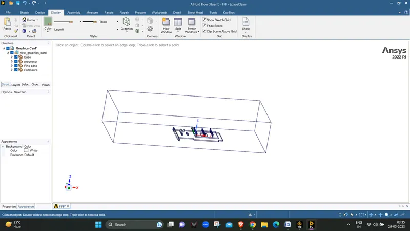
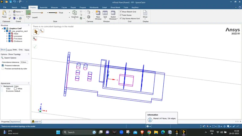
- so we will do share topology when its enabled a pink sign will apper showing that share topolody is enabled.
- Now we will move towards meshing module. with body sizing as 0.5 mm for whole graphic card and a seperate body sizing of 0.1 mm for the two cylinders on the base.
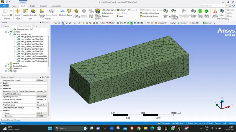
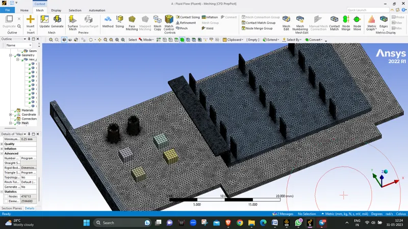
- the fine mesh is created near to the graphic card with total number of element count as 2627583..
- now we will give name selections to the whole body.
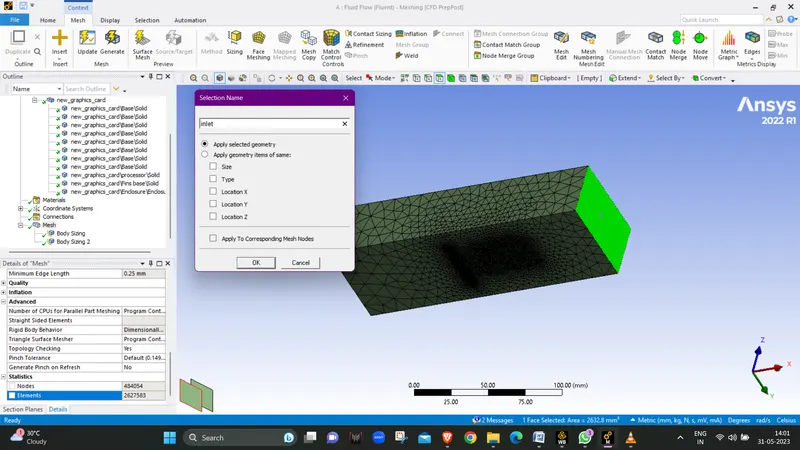
- Inlet :-
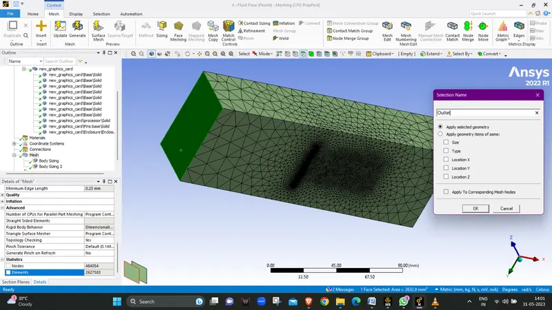
- Outlet :-
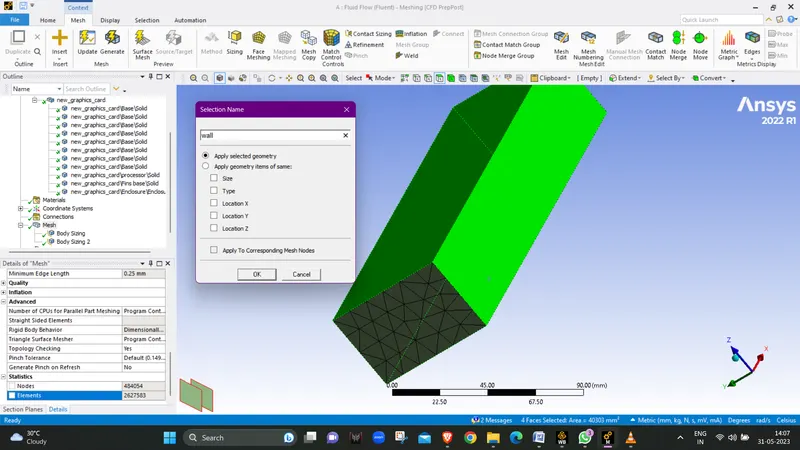
- Wall:-
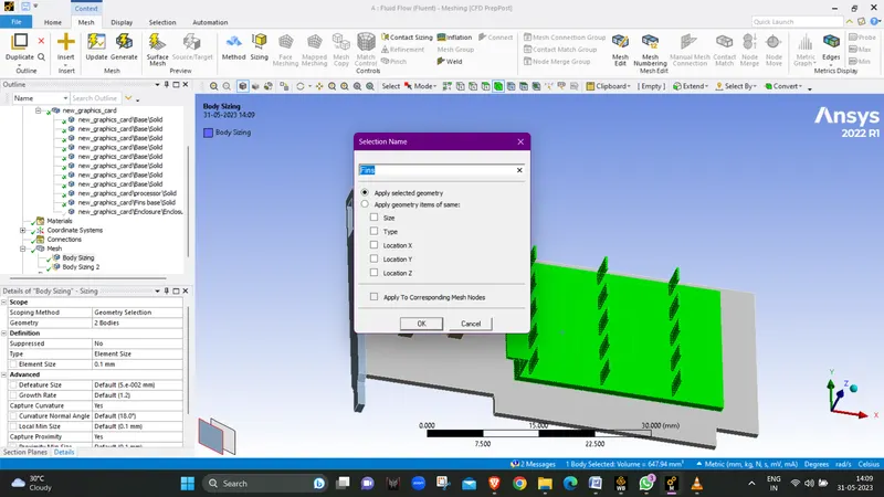
- Fins :-
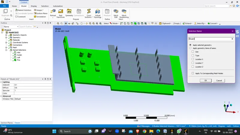
- Board:-
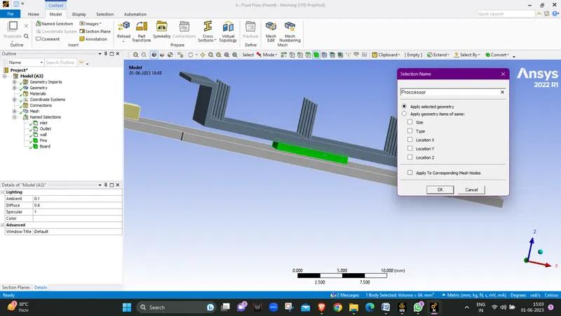
- Processor :-
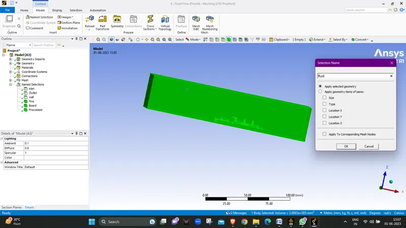
- Fluid :-
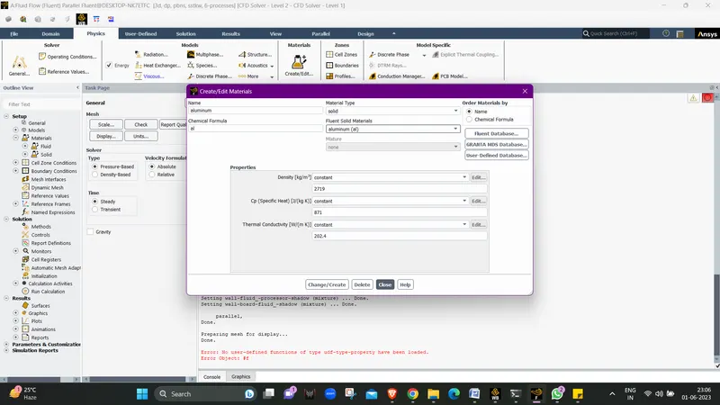
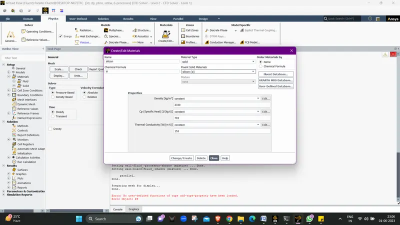
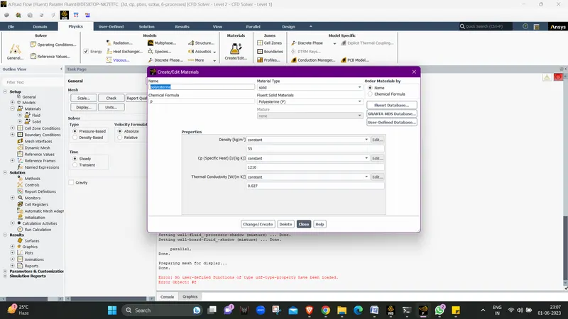
Now we will move towards the Setup Window and enable the Energy by checking he tick mark and then add new materials to the meterials list by copying one matrial properties and naming them as other material and after that changing the properties for the desired meterial properties.
- Aluminium :-
- Silicon :-
- Polyesterine :-
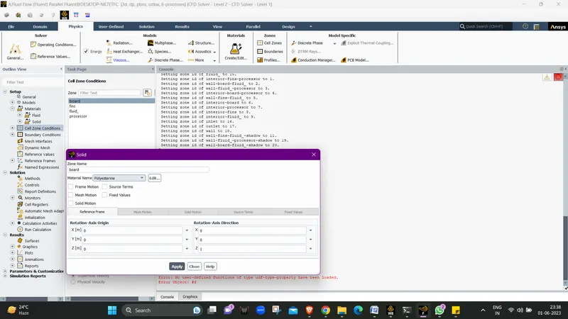
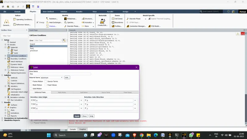
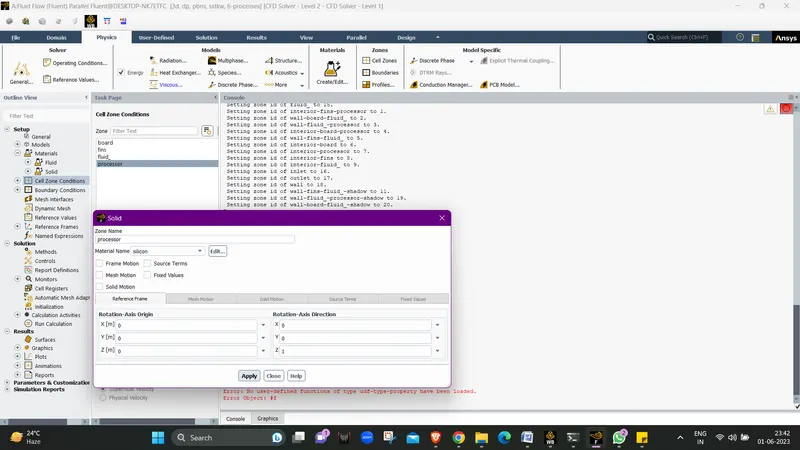
- Now we will setup the Cell Zone Conditions for the body with assigning material to them.
- Board material as Polysterine.
- Fins material as Aluminium.
- Processor material as Silicon.
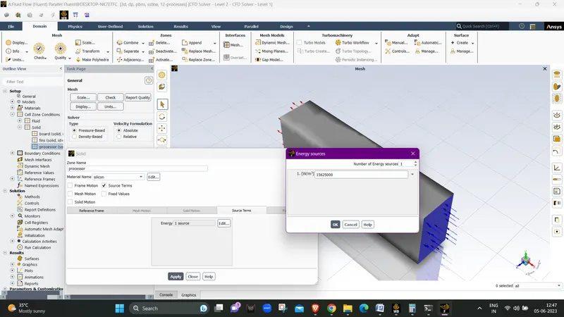
- In the proceesor cell zone condition we will click on Source terms check box which will activate the Source terms bar click on edit put the value 1 and then a new window pops up enter the value that we calculated for heat generation rate as 15625000 W/m3 and click ok and apply.
- Now we will give the boundary conditions for the simulation in which we will be giving inlet as 1m/s for first case.
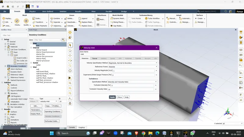
- we forget to add the input parameters in the inlet conditions. so we will add it now.
- we wil open inlet conditions and click on the drop down arrow where we added the velocity value and click on New Input Parameter which open a new window where we will add the new name as Velocity_Input and add 1m/s as inlet velocity.
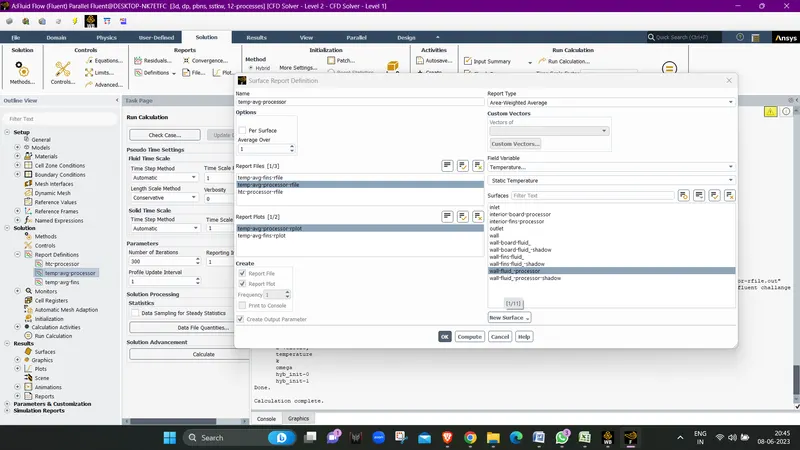
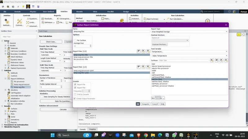
- Now we will make report definations with adding output parameter in the report defination by checking the option Create Output Parameters in report definatons.
- HTC on wall-fluid_Processor.
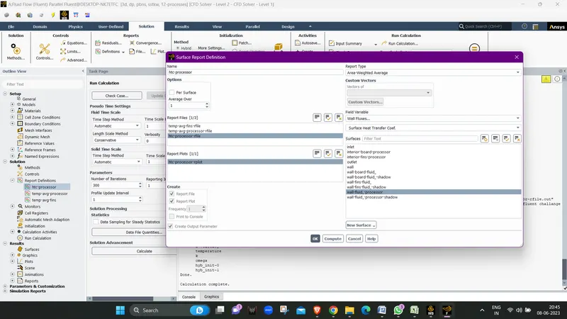
- Temp-avg-processor :-
- Temp-avg-fin
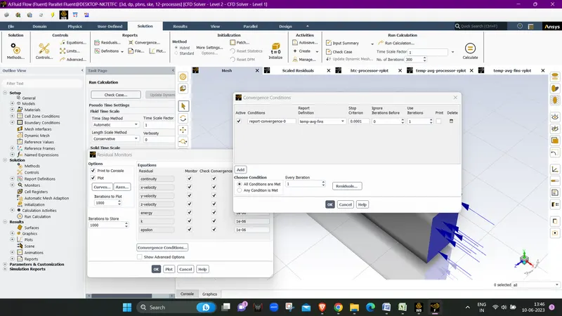
- Now we will hybrid initialize and run the calculation with setting convergence condition for fin temprature and make sure that the turbulance model we select is K omega SST model as it is suitable for both heat teansfer and flow conditions.
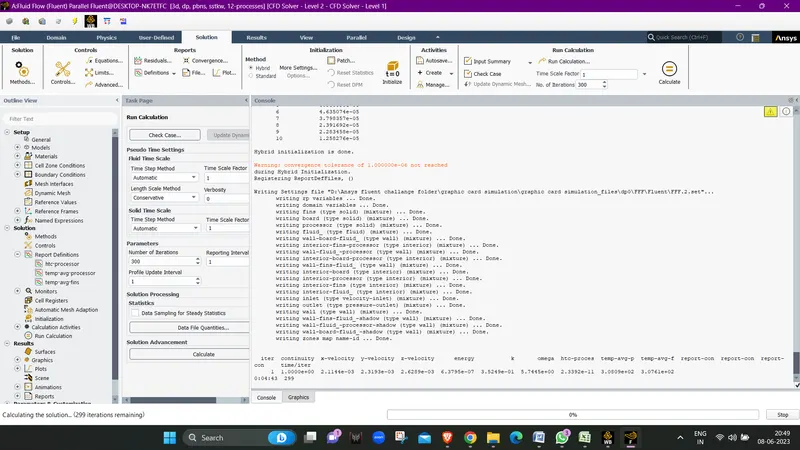
- and now we will run the solution by clicking on Calculate.
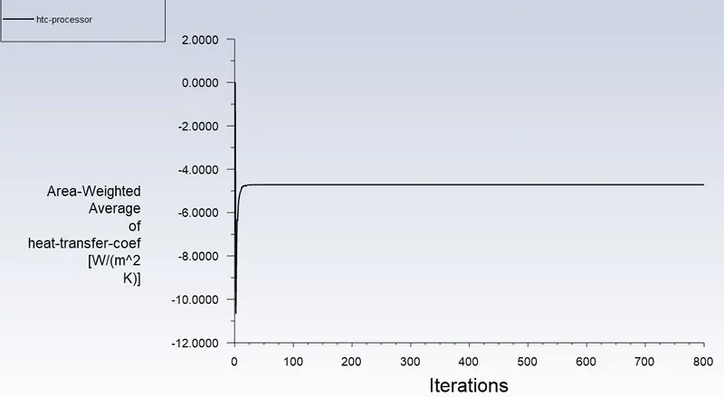
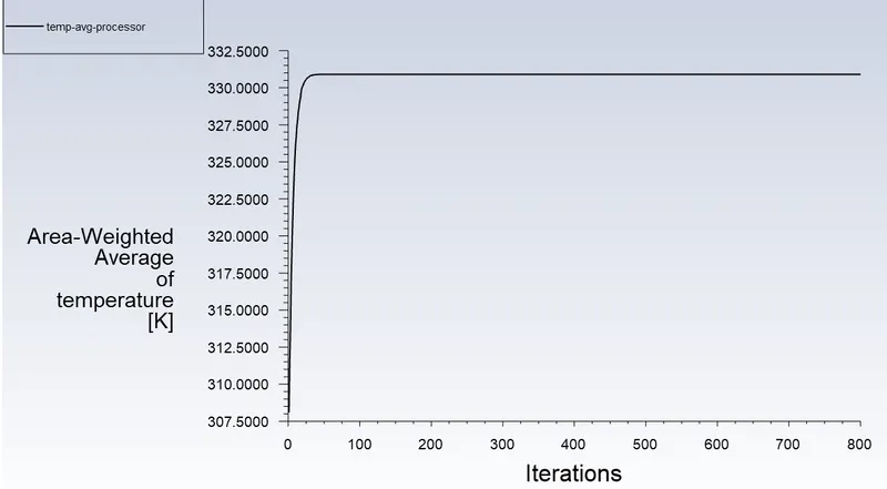
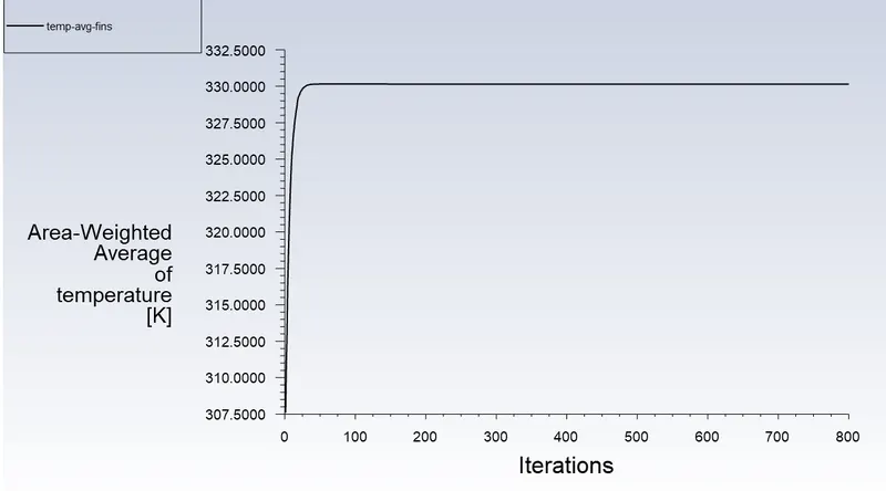
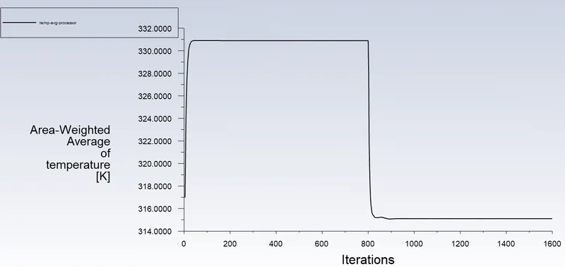
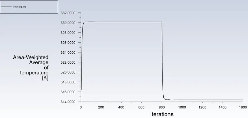
- Now we will get the result plots for heat transfer coefficient for processor and average temprature for both the find and temprature.
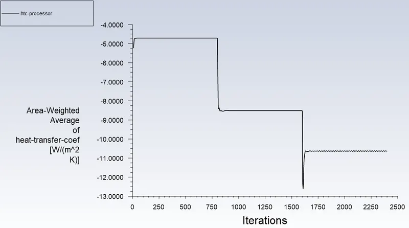
- Htc_Processor_plot
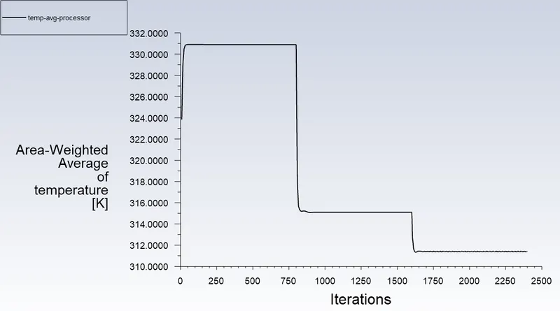
- Temp_Avg_Processor :-
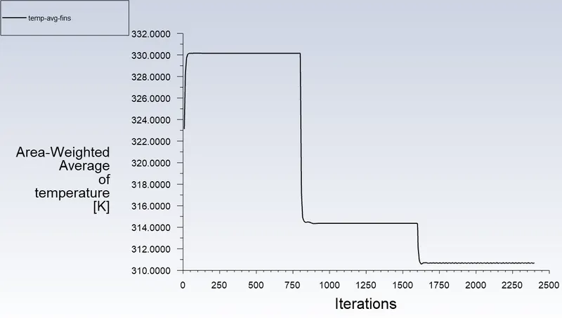
- Temp_Avg_fin :-
- Scaled Residuals :-
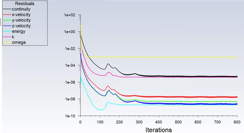
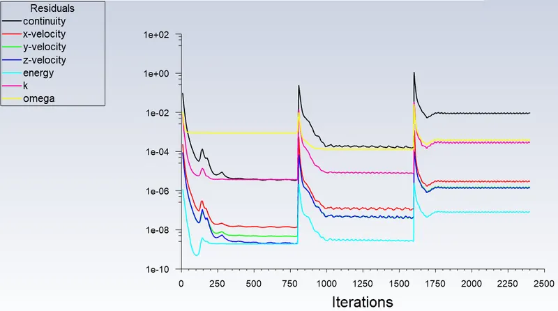
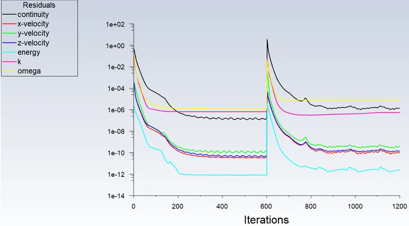
- We can see allt he values are converged in the plots so lets compute the final average values for the simulations.
- Htc_Processor :- -4.7125 [W/(m^2 K)].
- Temp_Avg_Processor :- 330.9 K.
- Temp_Avg_Fin :- 330.5 K.
Now we will run the same analysis for 2 more casses and another 3 cases with changed direction of enclosure. and then we will compare the values of both the enclosures.
Report plots :-
Enclosure 1 :- Flow of air in x direction :-
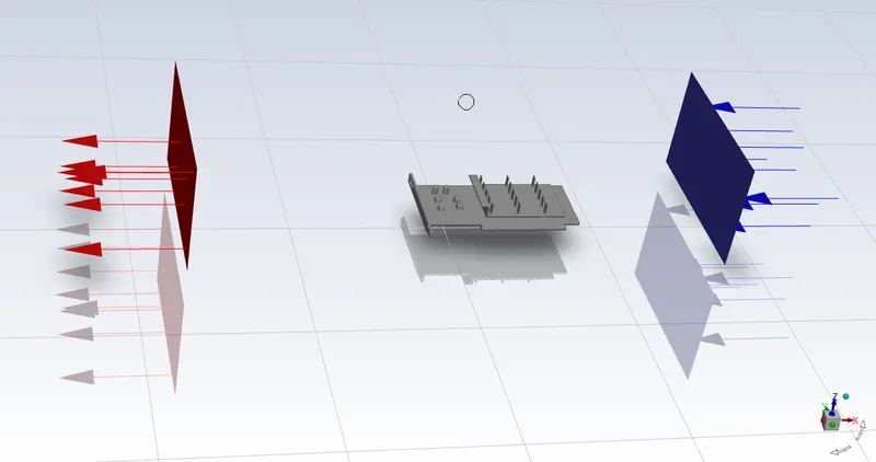
case 1 :-
Inlet velocity (1 m/s)
Residual plot :-
Htc_Processor_plot :-
Temp_Avg_Processor :-
Temp_Avg_fin :-
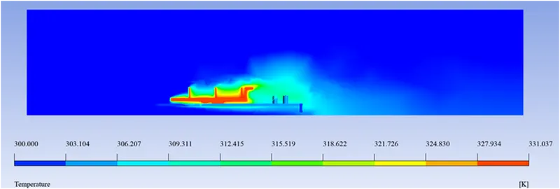
Temp Contour :-
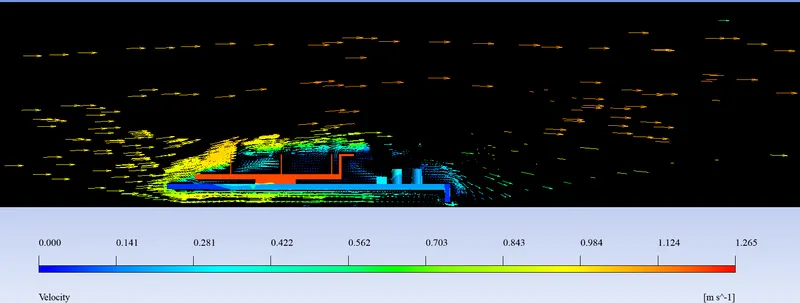
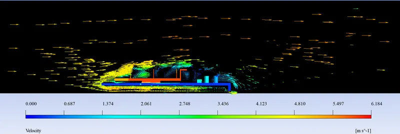
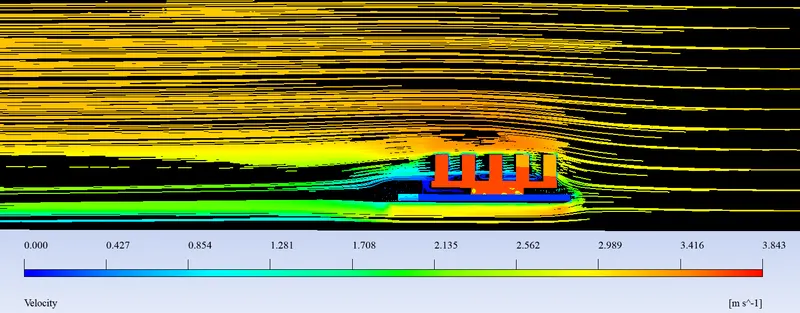
Velocity Vector Contour :-
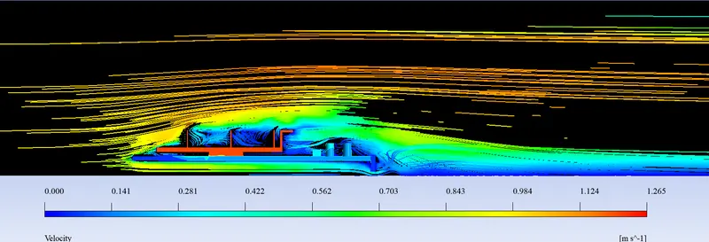
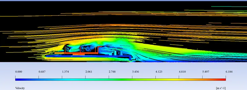
Velocity Streamline Contour :-
Enclosure 1 :- Flow of air in X direction :-
case 2 :-
Inlet velocity (3 m/s)
The plot starts from 800 th iterations
Residual plot :-
Htc_Processor_plot :-
Temp_Avg_Processor :-
Temp_Avg_fin :-
Temp Contour :-
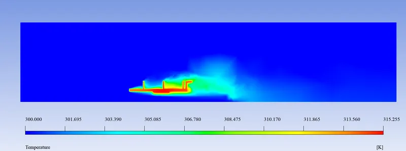
Velocity Vector Contour :-
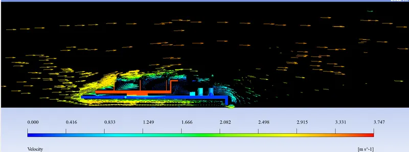
Velocity Streamline Contour :-
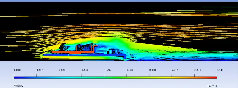
Enclosure 1 :- Flow of air in X direction :-
case 3 :-
Inlet velocity (5 m/s)
The plot starts from 1600 th iterations
Residual plot :-
Htc_Processor_plot :-
Temp_Avg_Processor :-
Temp_Avg_fin :-
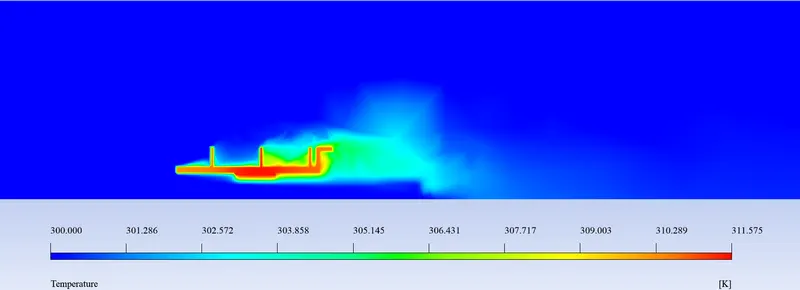
Temp Contour :-
Velocity Vector Contour :-
Velocity Streamline Contour :-
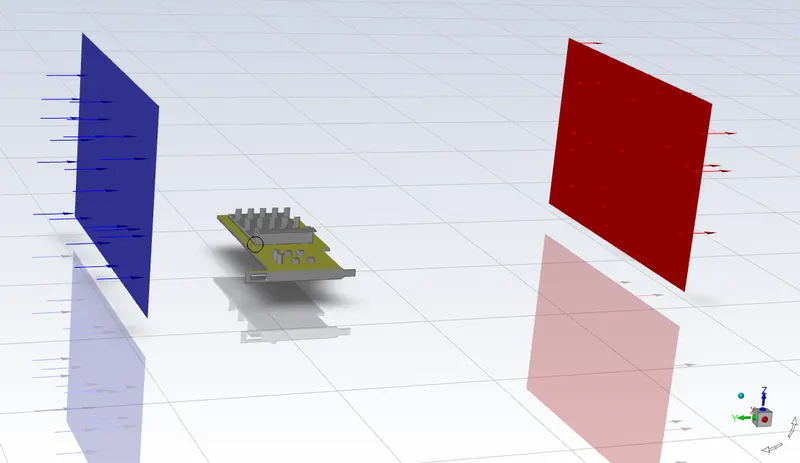
Enclosure 2 :- Flow of air in Y direction :-
Case 1 :-
Inlet velocity (1 m/s)
Residual plot :-
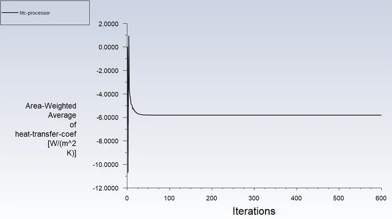
Htc_Processor_plot :-
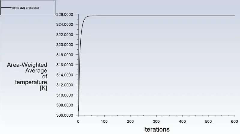
Temp_Avg_Processor :-
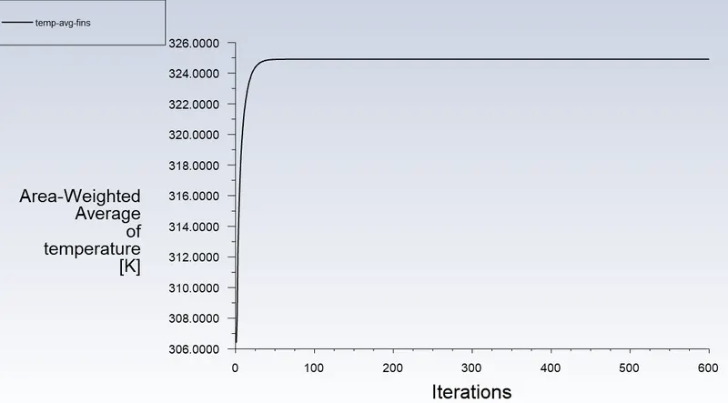
Temp_Avg_fin :-
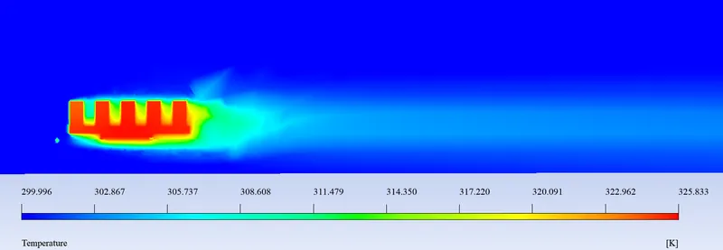
Temp Contour :-
Velocity Vector Contour :-
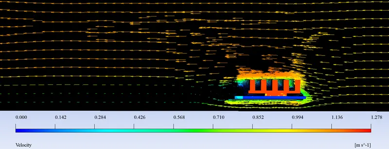
Velocity Streamline Contour :-
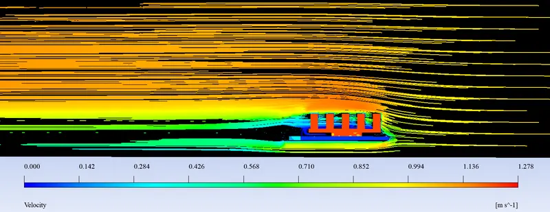
Enclosure 2 :- Flow of air in Y direction :-
Case 2 :-
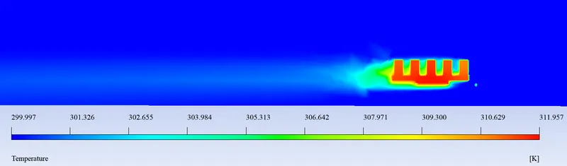
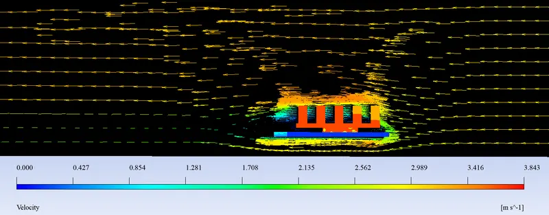
Inlet velocity (3 m/s)
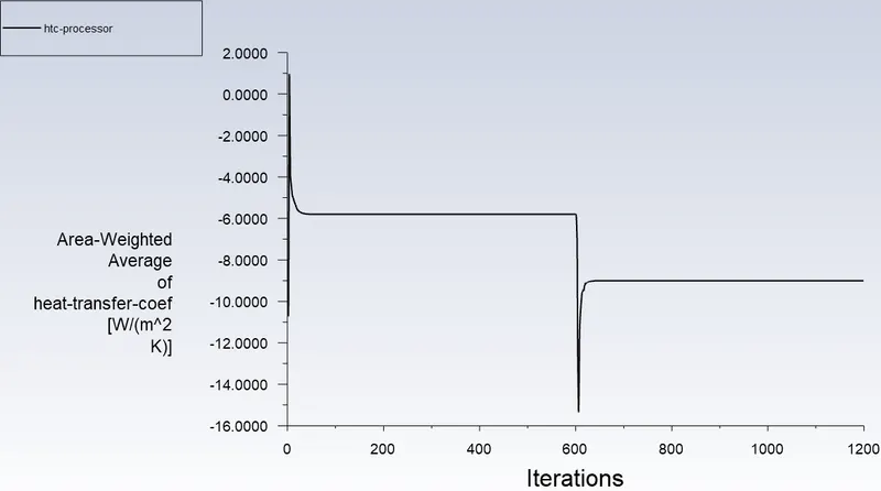
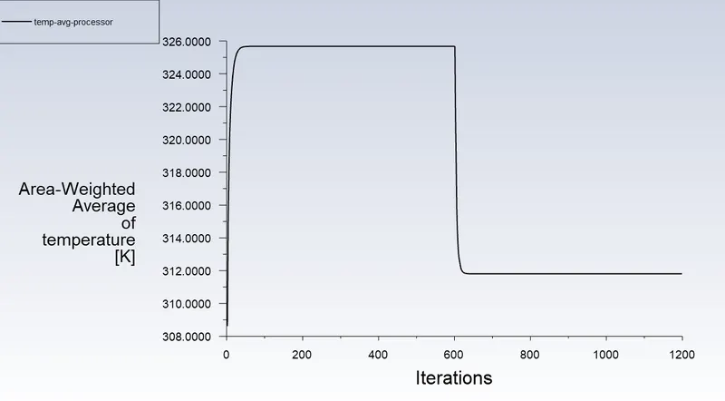
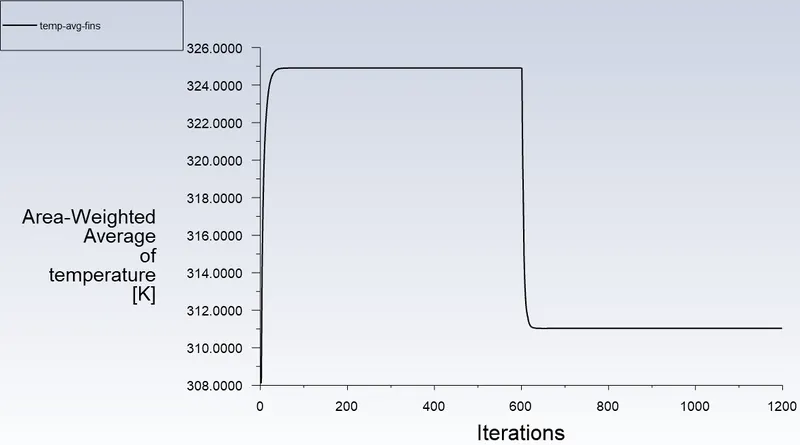
The plot starts from 600 th iterations
Residual plot :-
Htc_Processor_plot :-
Temp_Avg_Processor :-
Temp_Avg_fin :-
Temp Contour :-
Velocity Vector Contour :-
Velocity Streamline Contour :-
Enclosure 2 :- Flow of air in Y direction :-
Case 3 :-
Inlet velocity (5 m/s)
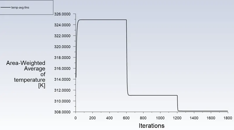
The plot starts from 1200 th iterations
Residual plot :-
Htc_Processor_plot :-
Temp_Avg_Processor :-
Temp_Avg_fin :-
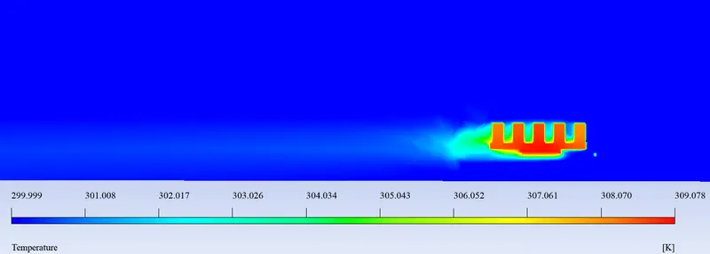
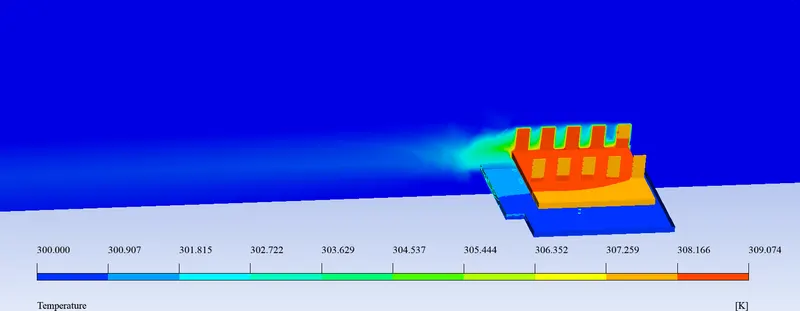
Temp Contour :-
Velocity Vector Contour :-
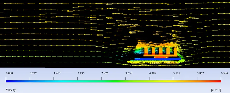
Velocity Streamline Contour :-
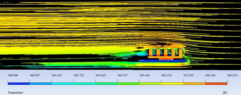
Now we will analyse the result an see what conclusion we have.
Results :-
|
S.No. |
Enclosure |
Cases |
Velocity (m/s) |
HTC (W m-2 K-2) |
Temp_Processor (k) |
Temp_Fin (k) |
|
1 |
Enclosure 1 |
Case 1 |
1 |
-4.7124952 |
330.897 |
330.146 |
|
2 |
Case 2 |
3 |
-8.5111463 |
315.103 |
314.366 |
|
|
3 |
Case 3 |
5 |
-10.655007 |
311.428 |
310.704 |
|
|
4 |
Enclosure 2 |
Case 1 |
1 |
-5.8003354 |
325.676 |
324.910 |
|
5 |
Case 2 |
3 |
-9.0004233 |
311.812 |
311.034 |
|
|
6 |
Case 3 |
5 |
-9.5670898 |
308.936 |
308.163 |
we can see from the above table in both enclosures the temp for processor have decreases with rising velocity which is due to higher het dicipation from the processor surface to the air with increse in velocity of air.
And if we compare the Enclosure 1 and Enclosure 2 we can see that the results we get for enclosure 2 are better than Enclosure 1 we can compare from the above table and from the temp plots of both the enclosure. let take any two cases with same velocity lets take the maximum velocity.
Case 3 of both enclosure we can see that temprature difference in both the case for temprature of processor is around 2.876 k so in case for enclosure 2 the temprature is less at processor than enclosure 1 and same
if we see for the temprature of fin for the both cases we get a temp difference of 2.871. so we can see again the temprature of fin is sless for enclosure 2 from above enclosure . so frome here we can see that heat dicipation is more in case of enclosure 2.
lets see the temp plots for both the enclosures.
Enclosure 1 Case 3 temp plot :-
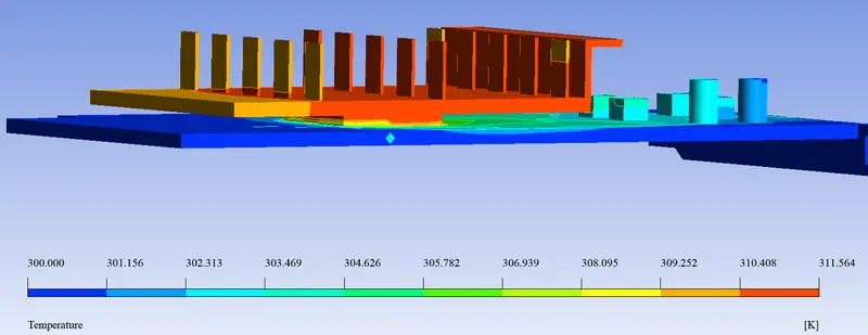
we can assume the minimum temp for fin and processor as 309.83 k
Enclosure 2 Case 3 temp plot :-
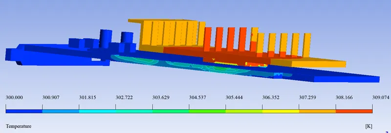
we can assume the minimum temp for fin and processor as 307.71 k
So we can see from both the temprature contours that the enclosure 2 is better than enclosure 1 for heat discipation over a graphic card. ans higher velocity is preferable and one more thing we can do decrease the temprature of the inlet air using a collant pipe so the heat discipation will be more.