Week 6 - CHT Analysis on a Graphics card

AIM:

Perform a steady-state conjugate heat transfer analysis on a model of a graphics card using appropriate materials of your choice for the simulation. Make sure to properly define the correct solid and fluid zones.

Run the simulation for the best possible mesh with a combination of coarse and refined mesh in different regions. Explain the reason for choosing the particular mesh settings.

Expected results:

• Run the simulation by varying the velocity from 1m/sec to 5m/sec for at least 3 velocities and discuss the results.
• Run the simulation by changing the flow pattern and discuss the results.
• Find out the maximum temperature and heat transfer coefficient obtained by the processor.
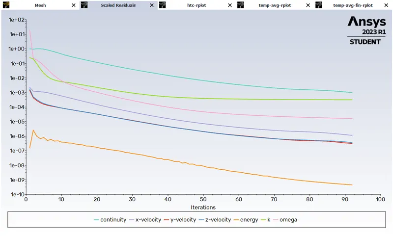
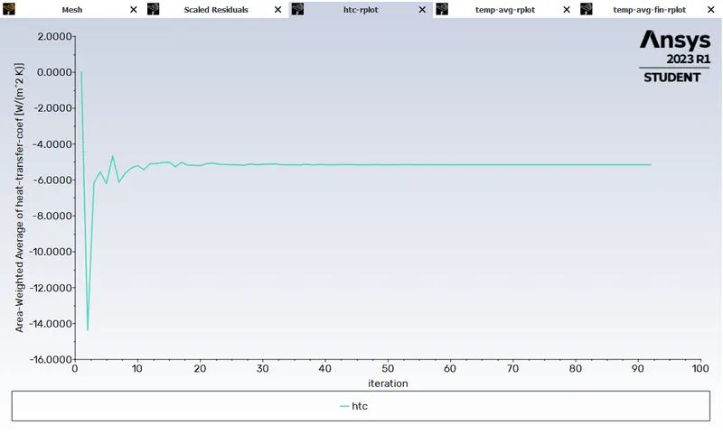
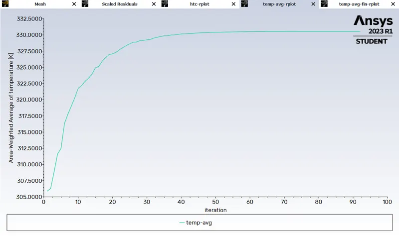
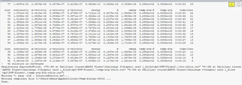
• Prove that the simulation has achieved convergence with appropriate images and plots.
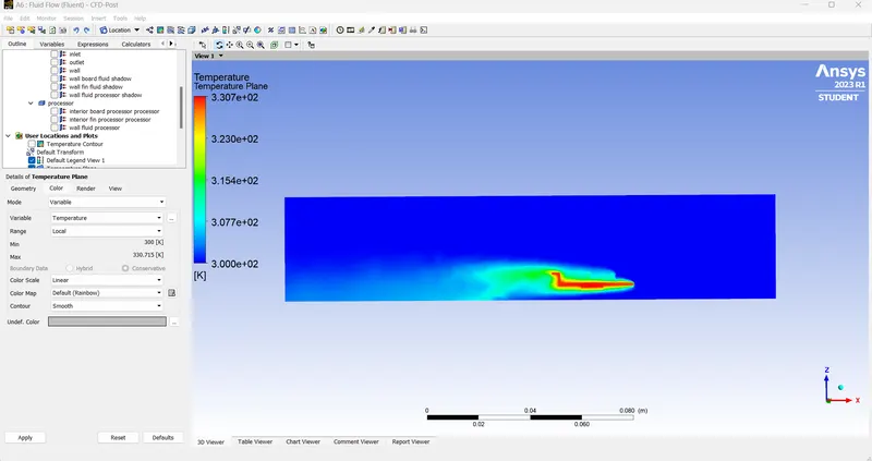
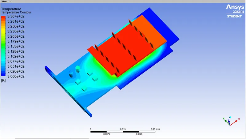
• Identify potential hotspots on the model.

INTRODUCTION:

Computational Heat Transfer (CHT) analysis on graphics cards plays a crucial role in understanding and managing the thermal behavior of these powerful computing components. Graphics cards, also known as GPUs (Graphics Processing Units), are widely used in various applications such as gaming, computer graphics, artificial intelligence, and scientific simulations. Due to their intensive computational capabilities, graphics cards generate substantial heat during operation, which can adversely affect their performance, reliability, and lifespan.

CHT analysis focuses on studying the heat transfer phenomena within graphics cards, encompassing the thermal interactions between the GPU chip, memory modules, power delivery components, and the surrounding environment. By employing mathematical models and simulation techniques, CHT analysis allows engineers to predict and optimize the thermal performance of graphics cards, ensuring efficient cooling and preventing overheating issues.

CHT analysis typically involves solving the heat transfer equations, such as the steady-state or transient conduction equations, within the graphics card domain. These equations take into account heat conduction through solid materials, convection at the surfaces, and radiation if applicable. Boundary conditions, such as heat sources, temperature constraints, and cooling mechanisms, are defined to simulate the real-world operating conditions.

THEORY:

Heat Transfer Coefficient:

The heat transfer coefficient is a fundamental parameter in heat transfer analysis that quantifies the rate of heat transfer between a surface and a fluid (gas or liquid). It represents the effectiveness of the heat transfer process and is defined as the amount of heat transferred per unit area per unit temperature difference between the surface and the fluid.

Mathematically, the heat transfer coefficient (h) is expressed as:

Q = h × A × ΔT

Where, Q is the heat transfer rate, A is the surface area in contact with the fluid, and ΔT is the temperature difference between the surface and the fluid.

SOLVING & MODELLING APPROACH:

In this simulation, working fluid i.e. air, is flown over a graphics card from inlet part of an enclosure as it is an internal analysis at a velocity of 1 m/s, 3 m/s and 5 m/s respectively to the outlet part of the enclosure. K-omega SST model is used for this simulation as it gives better results for analysis near the wall and to capture the flow properly. Materials such as Aluminum (Al), Silicon (Si) and Polysterene (P) is used for Fins, Processor and the board respectively.

PRE-PROCESSING AND SOLVER SETTING:

Geometry:

• Run ANSYS 2023 R1 student version and drag Fluid Flow (Fluent) in the project Schematic and then run ANSYS Space Claim by selecting it from Geometry. Then import the Exhaust port by using the option File> Open>Graphics Card.stp

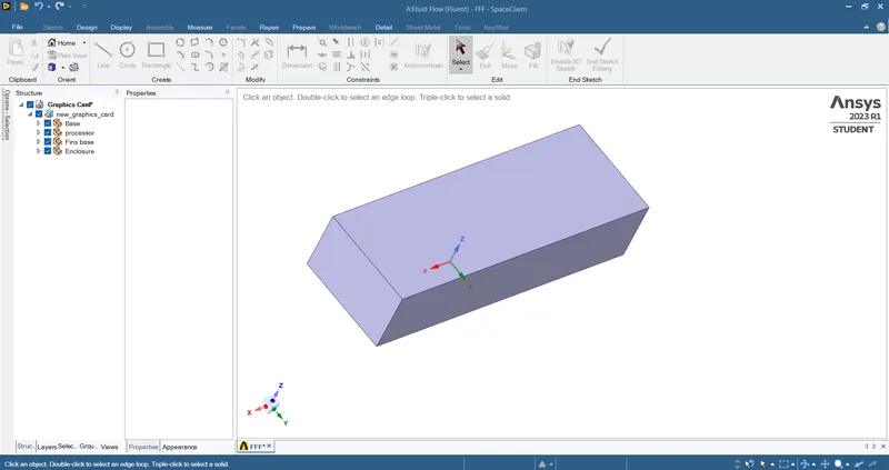
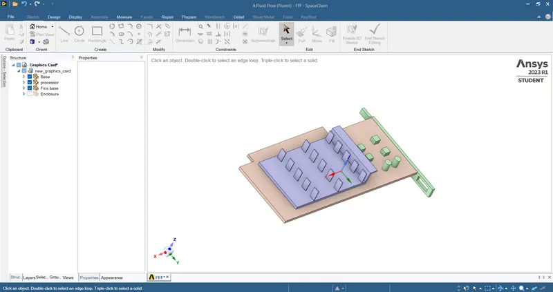
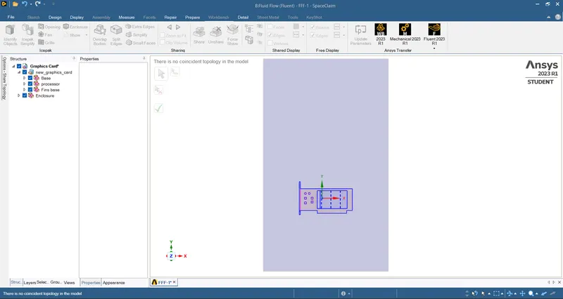
• Share topology between the enclosure and the graphics card so that the flow between them is achieved properly and meshing will be properly connected between them.

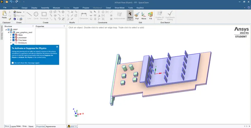
• For another case, create a new enclosure for changing the flow pattern and share the topology. The flow of the fluid will be from bottom of the enclosure to the upward part.

Mesh:

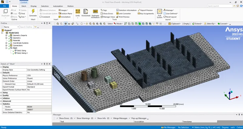
• Generate a coarse mesh after loading the graphics card in the meshing window with an element size of 10 mm. Then create different body sizing mesh for the different components in the graphics card because the processor is the heat generating source in the graphics card and so fine mesh is required near the processor and as heat transfer will take place between the processor and the fins where proper analysis is required to capture the fluid flow so the mesh elements in the fins and the processor will be more refined. Body sizing mesh element is taken as 1 mm for the board and the other bodies except the fins and the processor where the element size is taken as 0.5 mm. Inflation layer is not created for this simulation as it will exceed the number of mesh elements.

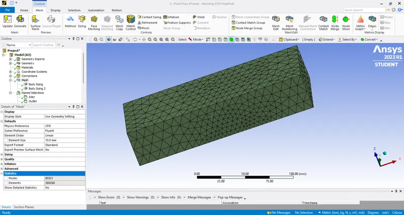
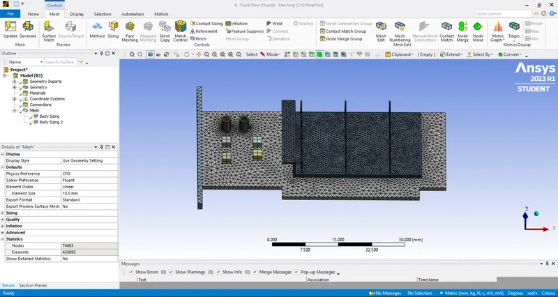
• Meshing for another case where the flow pattern is changed.

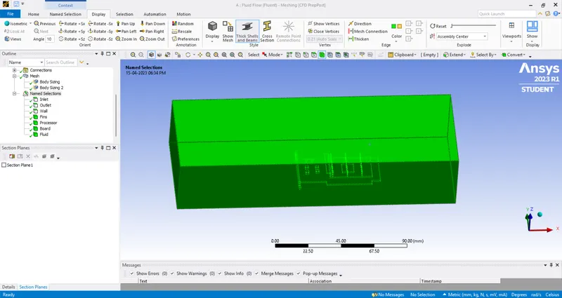
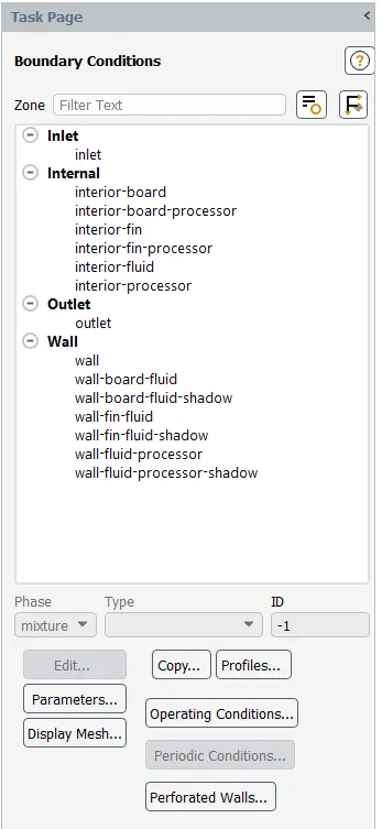
• Name the different sections of the geometric body such as inlet, outlet, wall, fluid domain, fin, processor and board by selecting the appropriate body/sides by using the named selection option or by clicking 'N" after selecting the side.

SETUP:

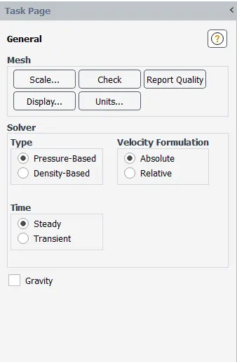
• Under general settings, selected pressure-Based type solver and steady time.

• Select Materials as air under fluid and create materials such as Aluminum for fins, Silicon for processor and Polysterene for board under solid and set boundary conditions, where the inlet velocity will be 1 m/s for the first case and then create parametric table for the inlet velocities to solve the simulation faster.

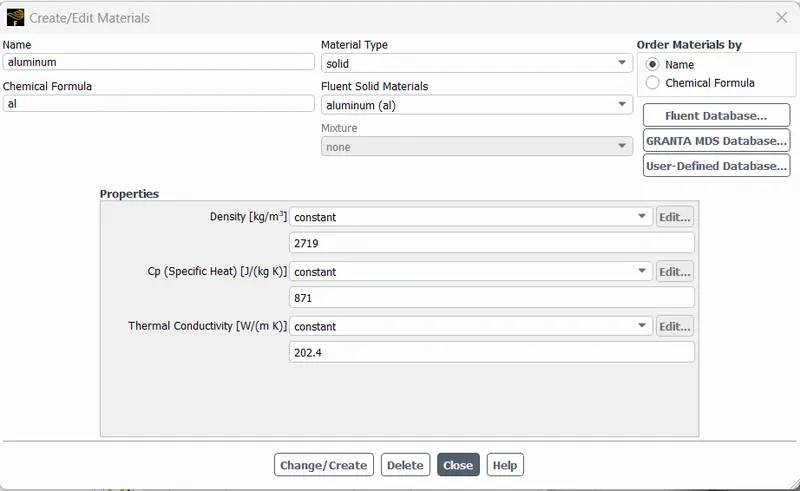
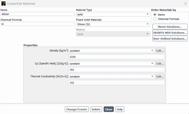
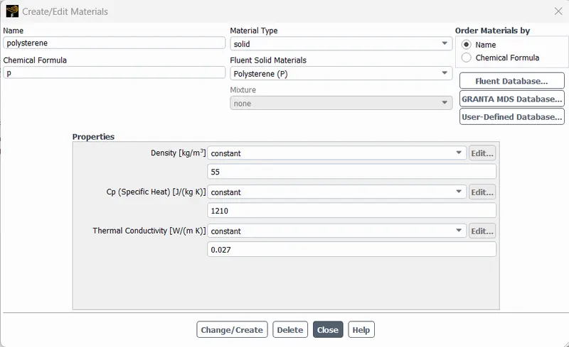
• Define cell zones for all the materials. Also select source terms for processor cell zone to provide the energy value of the processor i.e. the amount of heat produced.

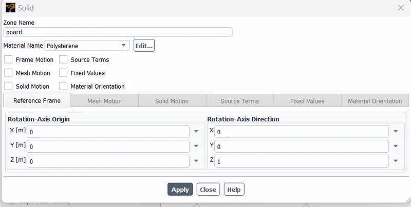
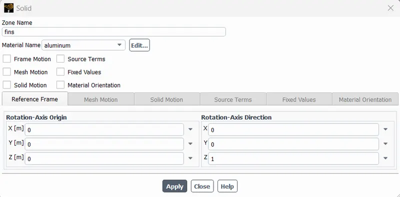
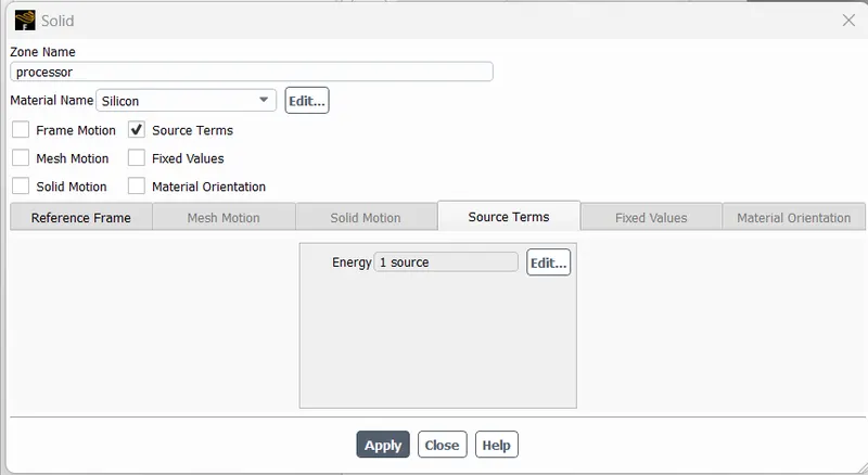
• Assign boundary conditions and make parametric table for assigning inlet velocities.

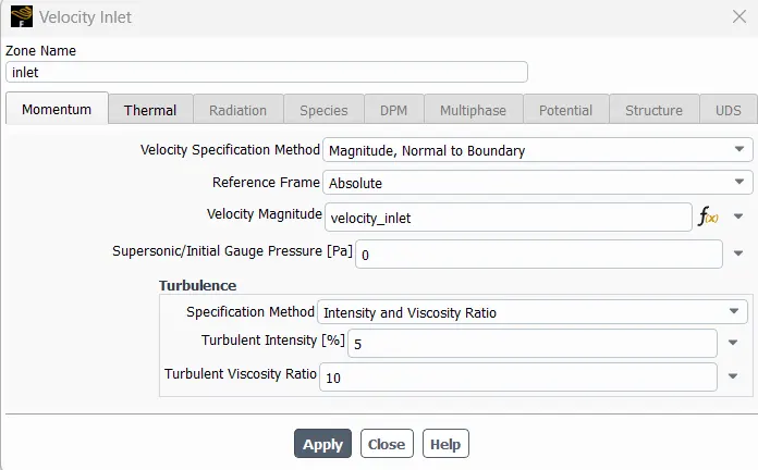
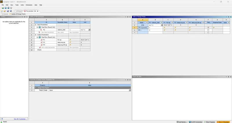
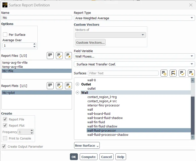
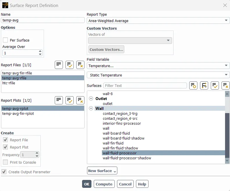
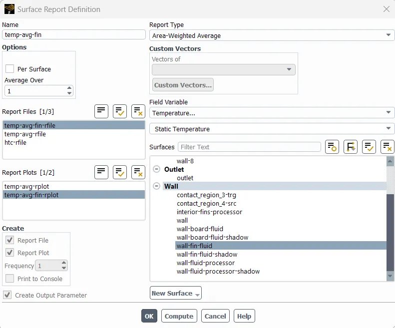
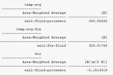
• Under solution tab, select Definitions> New>Surface Report>Area-Weighted Average and select Wall Fluxes and surface heat transfer coefficient for wall fluid processor, Definitions> New>Surface Report>Area-Weighted Average and select Temperature for wall fluid processor, Definitions> New>Surface Report>Area-Weighted Average and select Temperature for wall fin fluid to calculate heat transfer coefficient, average temperature in processor and fins respectively.

• For Initialization select Hybrid Initialization and then click initialize and then run necessary number of iterations until the solution is converged.

RESULTS:

For inlet velocity as 1 m/s:

Scaled Residuals:

Heat Transfer Coefficient Plot:

Temperature plots:

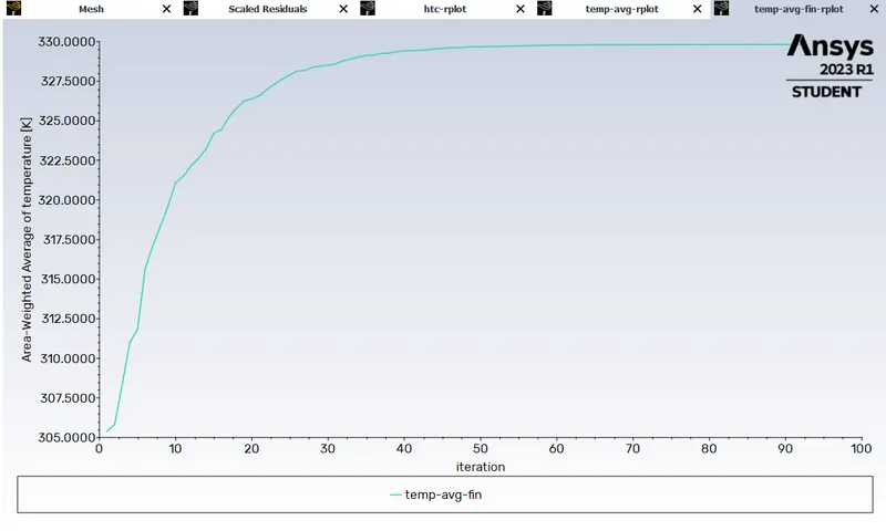
Converged solution:

Temperature contours:

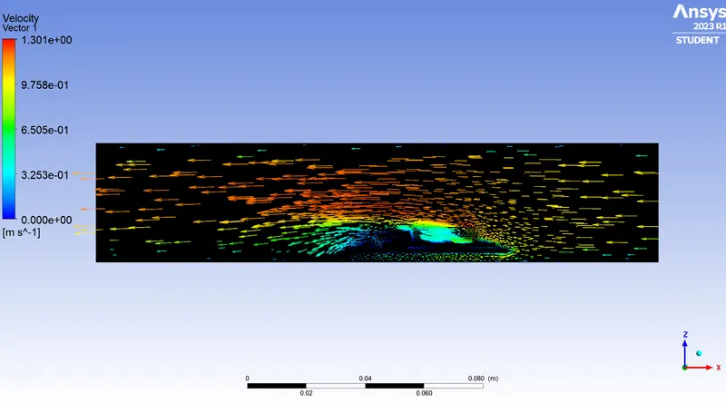
Velocity Vector:

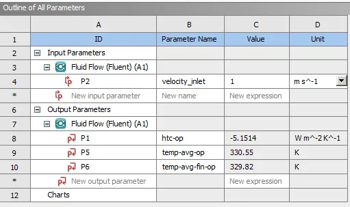
Results of report: Average Temperatures and Heat Transfer Coefficient

For inlet velocity 3 m/s:

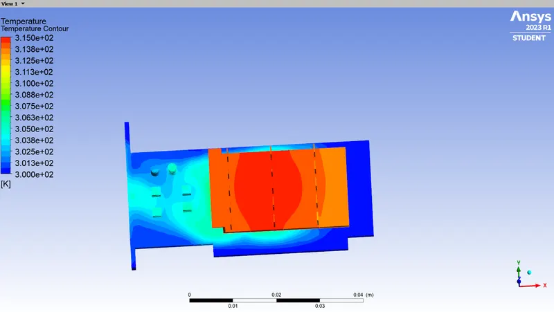
Temperature contour:

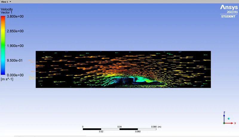
Velocity vector:

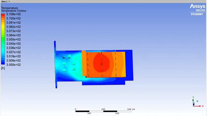
For inlet velocity 5 m/s:

Temperature contour:

Velocity vector:

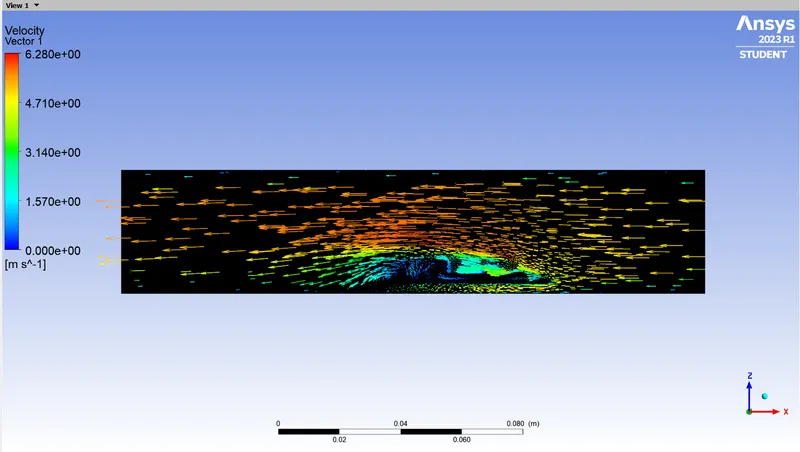
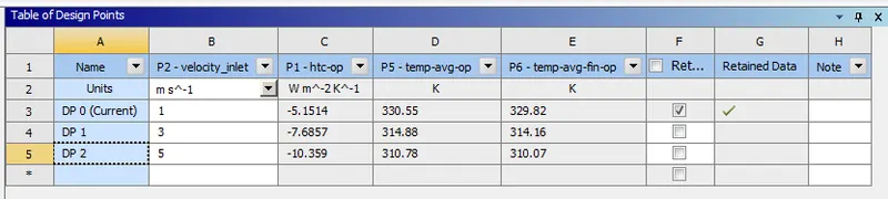
Table for Heat Transfer Coefficient, Average Processor Temperature and Average Fin Temperature where inlet velocities are 1 m/s, 3 m/s and 5 m/s respectively are as follows:

Results when the flow pattern is changed: For inlet velocity 1 m/s :

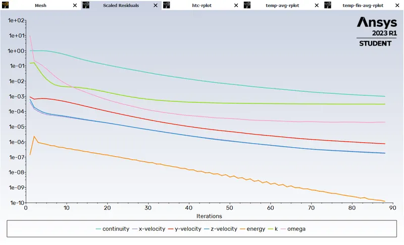
Scaled Residuals:

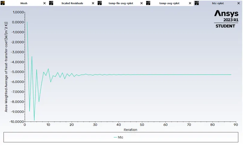
Heat Transfer Coefficient Plot:

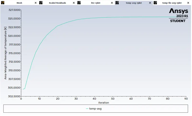
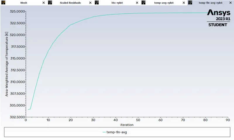
Temperature Plots:

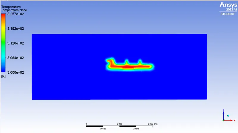
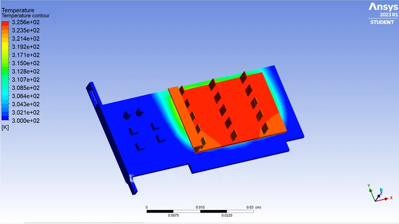
Temperature Contours:

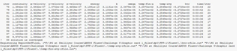
Coverged Solution:

Results of Reports: Average Temperatures and Heat Transfer Coefficient

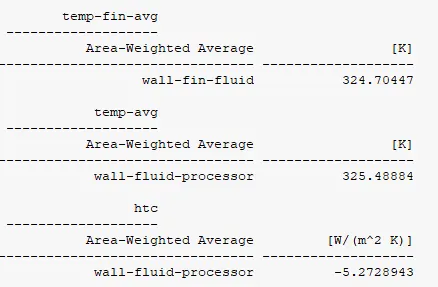
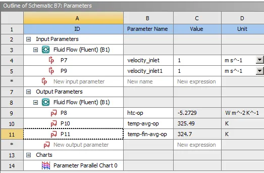
Table for Heat Transfer Coefficient, Average Processor Temperature and Average Fin Temperature where inlet velocities are 1 m/s, 3 m/s and 5 m/s respectively are as follows:

CONCLUSION:

• For the first case, The simulation has been run by varying the inlet velocities at 1 m/s, 3 m/s and 5 m/s respectively until the solution is converged. It has been observed that as the velocities increases the temperature decreases and the heat transfer coefficient increases as a result of which we can say that the heat transfer efficiency increases with increase in inlet velocity.
• For the second case, the simulation is also done by providing the same inlet velocities of 1 m/s, 3 m/s and 5 m/s until the solution is converged. It has been observed that with increase in inlet velocities there isn't a significant change in the temperatures when th flow pattern is changed, where as the heat transfer coefficient increases with increase in velocities.
• The maximum temperature and heat transfer coefficient of the processor is shown in tha above tables.
• The simulation has been properly converged as shown in the above images and plots.
• The potential hotspots are that the processor acts as the main heat source, with increase in inlet velocities heat transfer coefficient increases as a result the conduction and convection occurs with greater effeciencies, the more the mesh is refined, it leads much better results. The flow pattern for the first enclosure gives better results as the temperature decreases with higher velocities.