Week 6 - CHT Analysis on a Graphics card

AIM :- Conjugate heat transfer analysis on a graphics card.

OBJECTIVE:-

1. Run the simulation by varying the velocity from 1m/sec to 5m/sec for at least 3 velocities and discuss the results.
2. Find out the maximum temperature and heat transfer coefficient attained by the processor.
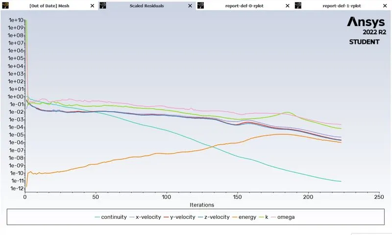
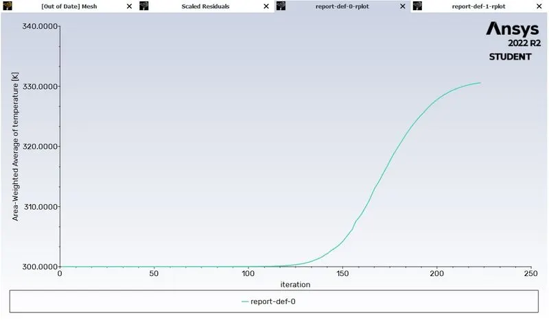
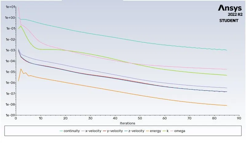
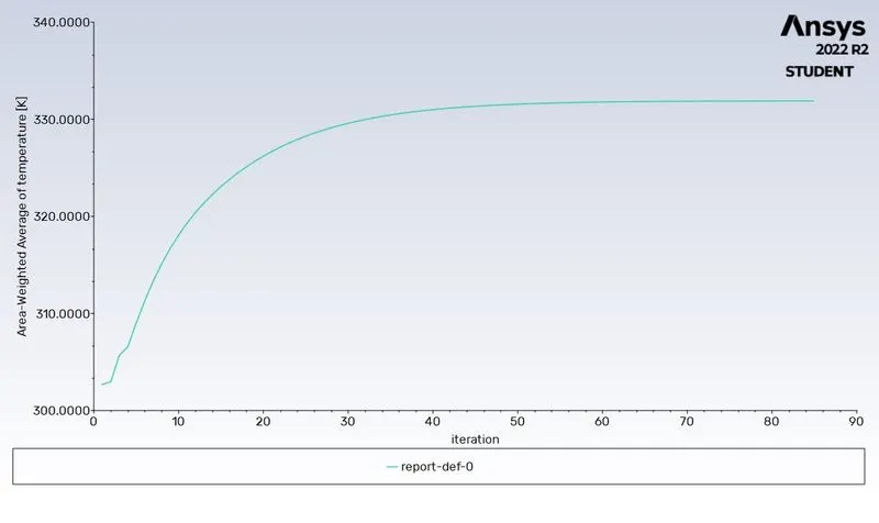
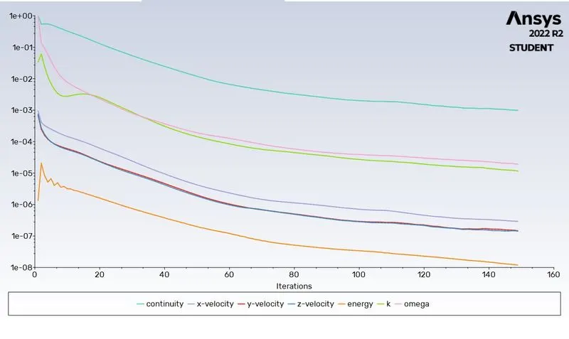
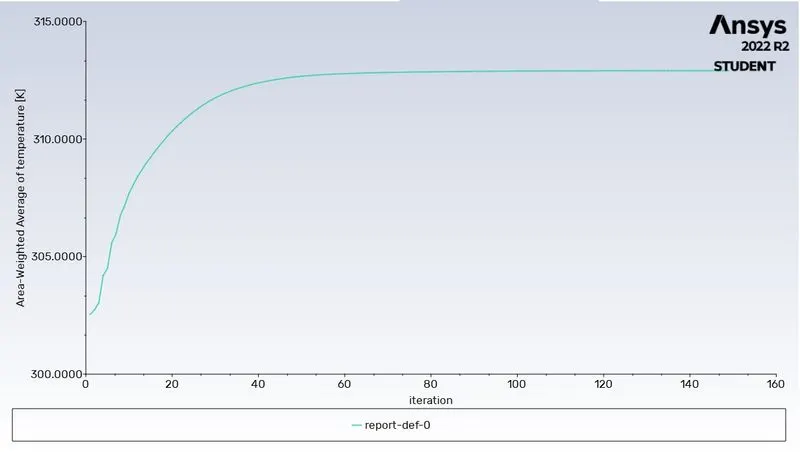
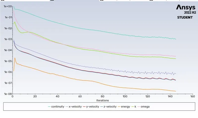
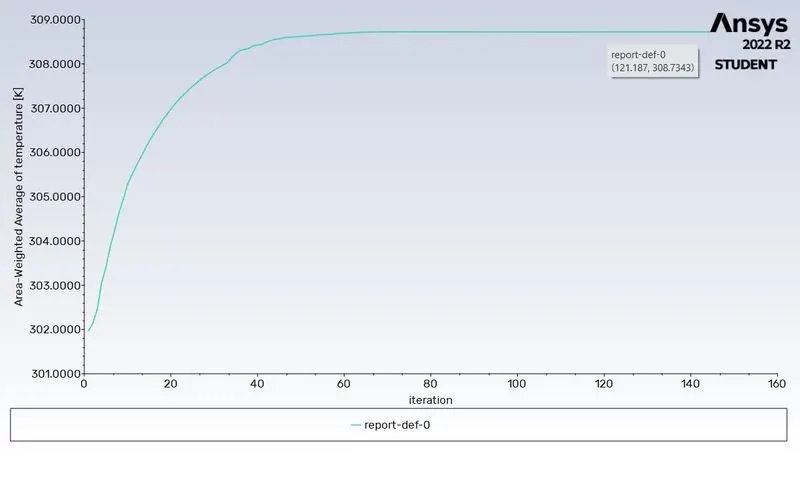
3. Prove that the simulation has achieved convergence with appropriate images and plots.
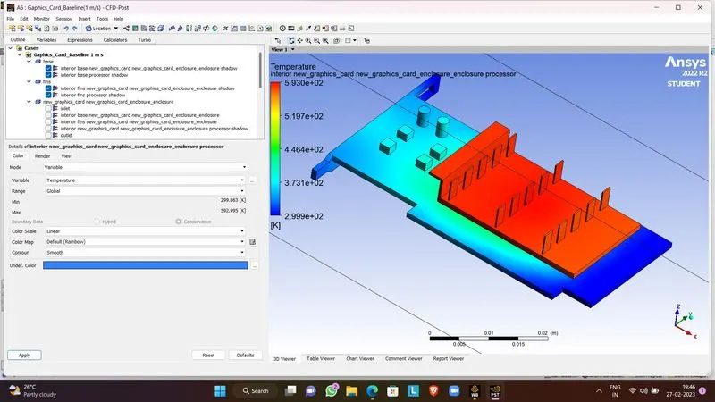
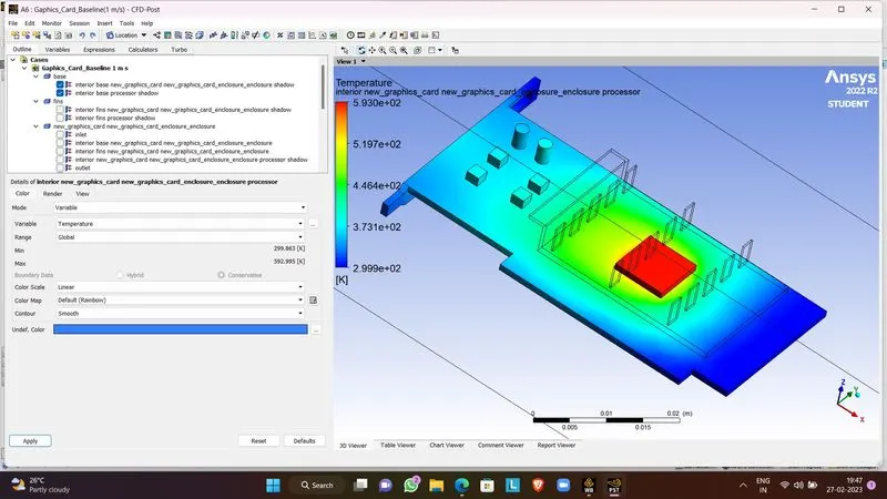
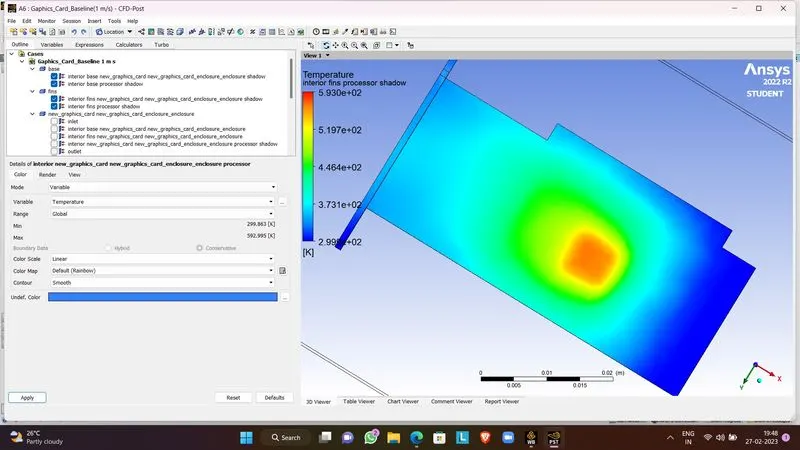
4. Identify potential hotspots on the model.

THEORY:

• Conjugate heat transfer:

Conjugate heat transfer is defined as the heat transfer between two domains by the exchange of thermal energy. For a system the thermal energy available is defined by its temperature and the movement of thermal energy is defined by its heat flux through the outer walls. Heat transfer in solid happens through conduction and in liquid phase through convection.

CHT provides the temperature prediction and the hotspot regions at the solid-fluid interface and we can also predict the heat transfer accurately for example- Conduction through solids, convection through fluid, and thermal radiation. It also provides the velocity and pressure distribution of fluid moving inside the solid. We can also use CHT in design optimization for the improvement of heat transfer and cooling capacity.

The Conjugate Heat Transfer (CHT) analysis type allows for the simulation of heat transfer between solid and fluid domains by exchanging thermal energy at the interfaces between them.

Examples:

HVAC, Heat Exchanger, Tank, Internal Combustion Engine, Heat Sink, Boiler, Reactor, Heat Pipe, Turbocharger.

• Geometry setup:

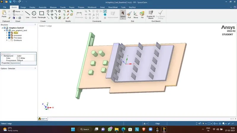
1. Use SpaceClaim to edit the geometry of the downloaded model of the graphics card which is in the enclosure.

2. Click on share prep to view any edges in interference so that conformal mesh can be achieved between different components.

3. Share topology has to be enabled between the different components so that necessary information can be shared between different zones of the mesh.

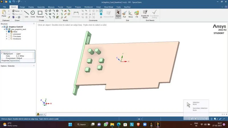
GRAPHICS CARD

BASE:

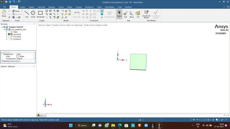
PROCESSOR:

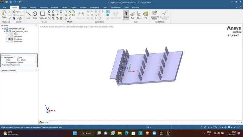
FINS:

• Mesh setup:

1. Before generating a base mesh, let's name the different components of the graphic card so it is easier to find them while setting up fluent.

2. Base, processor, and fins are basic name selections that will help us in the simulation.

3. Click generate mesh to create a base mesh, body sizing can be applied for the 3 solid components.

4. After creating the mesh, exit the Mesh setup to simulate in fluent.

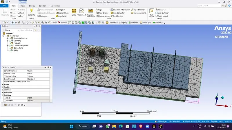
CASE 1.1. BASELINE MESHING (Coarse Mesh) :

Mesh Size: 5mm

No. of Elements: 1,64,767

No. of nodes: 31,547

SIMULATIONS

SETUP
Solver Type	Pressure-Based
Velocity Formulation	Absolute
Time	Steady
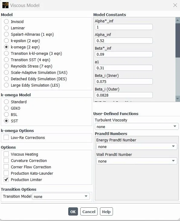
Models	Viscous model: K-omega SST Energy model: On
Material	Fluid type: Air Solid-type: Aluminium : FR-4 (Created) : Silicon (Created)
Cell zones	Fluid type: Air Solid: Al, fr-4, Si
Boundaries	Inlet: inlet velocity: 1m/s : temperature = 300K Outlet: outlet pressure = 0
Reference values	Standard
Initialization	Standard

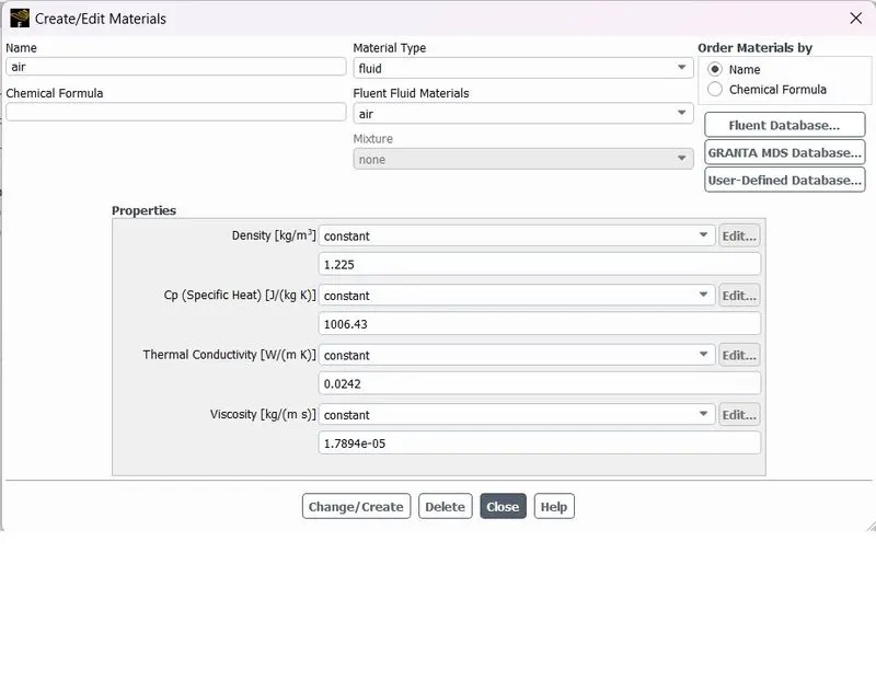
Materials :

We are using a different material for all the component

For fluid: Air

• Density = 1.225 kg/m^3
• Viscosity = 1.7894e-05 kg/ms

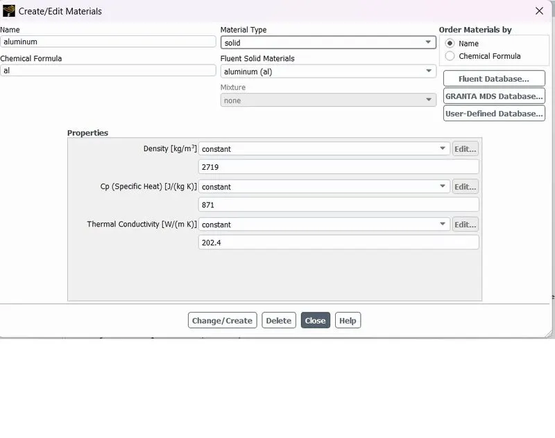
For Solid : Fins: Aluminium (Al)

• Density = 2719 kg/m^3
• Specific heat = 871 j/kg-k
• Thermal conductivity = 202.4 w/m-k

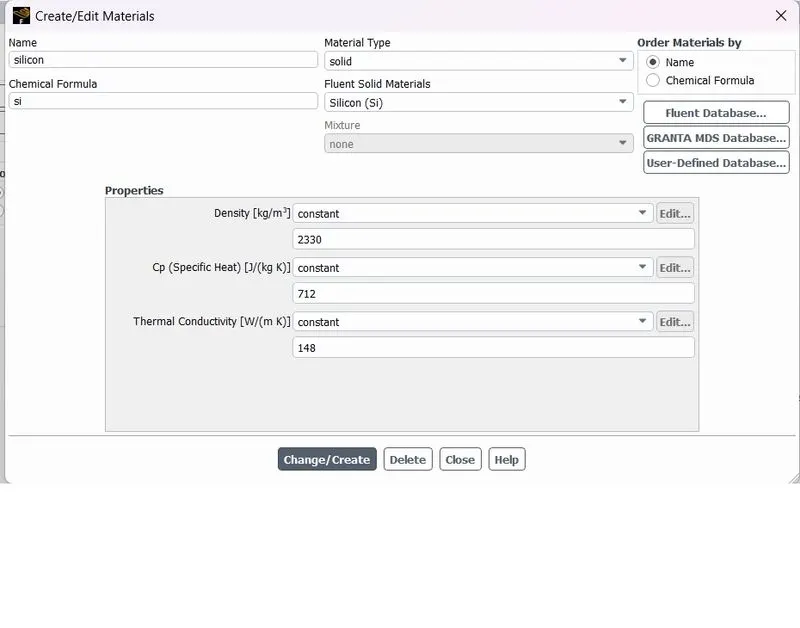
For Processor: Silicon (Si) (Created)

• Density = 2330 kg/m^3
• Specific heat = 712 j/kg-k
• Thermal conductivity = 148 w/m-k

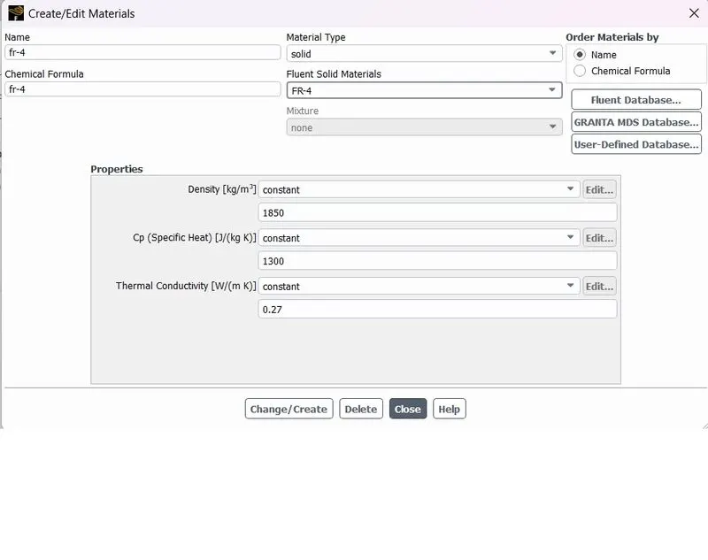
For Base: FR-4 (Created)

• Density = 1850 kg/m^3
• Specific heat = 1300 j/kg-k
• Thermal conductivity = 0.27 w/m-k

Setting up the source terms :

For this case, we consider that our processor is a source term and it generates heat.

So, for setting up the source term go to Zones - Cell zones - and click on the processor for editing which is in the Solid.

After that select the material to Silicon and click on the source terms to enable it and set the energy source to 1.

The calculation for the Energy source

Suppose the processor consumes 10 W of power to work.

Dimension of the processor = 8*8*1 mm^3

So, the Energy produced by the processor is 156250000 w/m^3.

RESIDUALS:

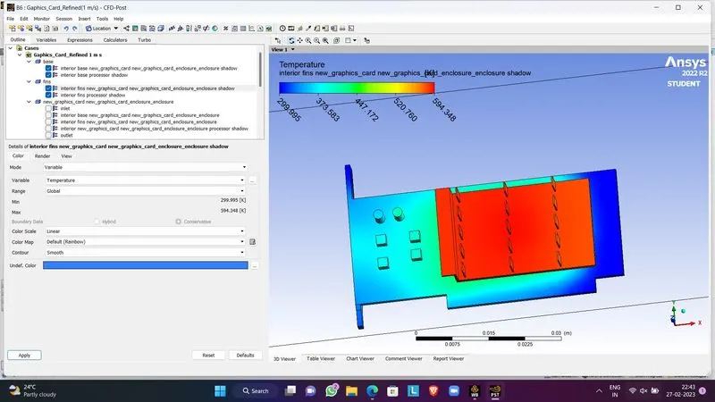
Global Hotspot region:

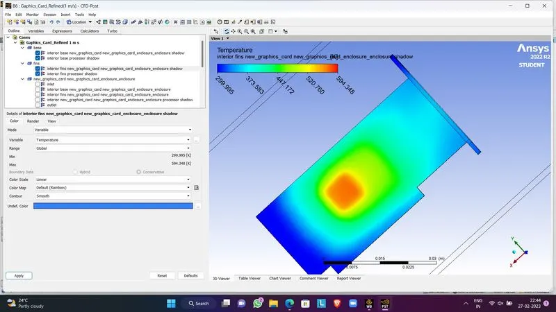
Local Hotspot around the processor:

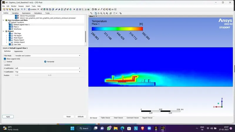
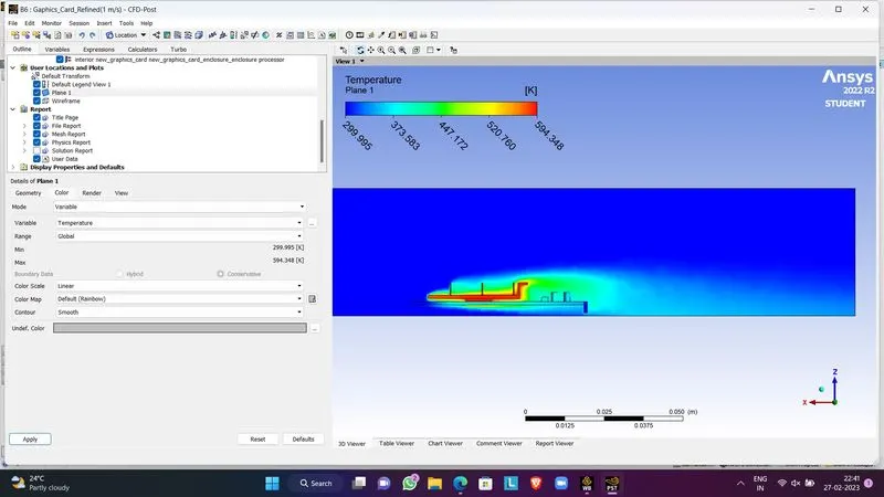
Temperature Contour:

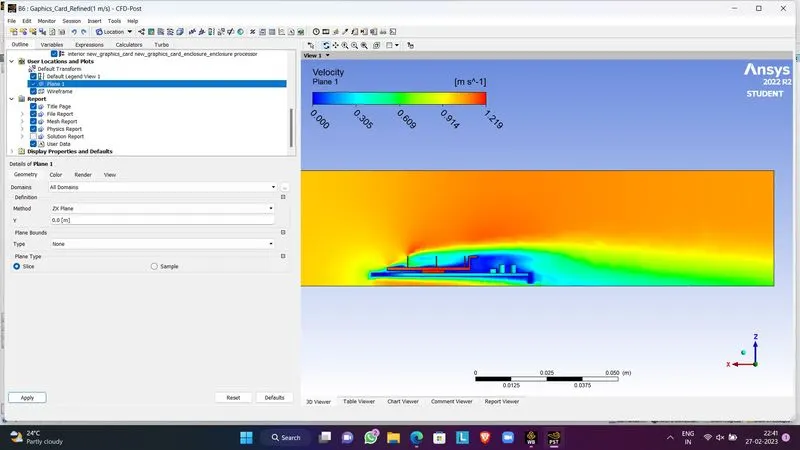
Velocity Contour:

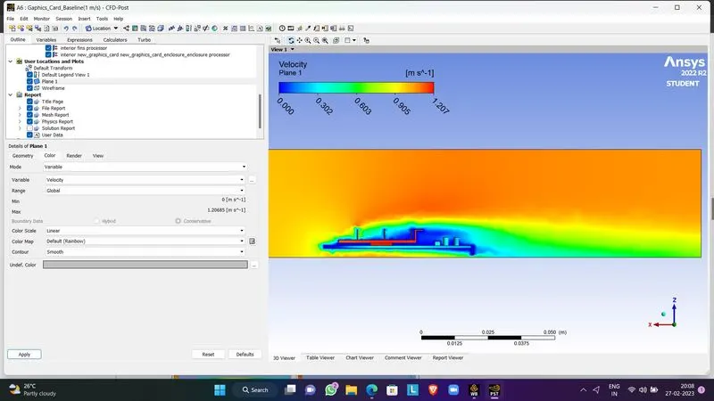
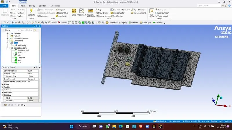
CASE: 1.2: REFINED MESH :

Base – 3 mm

Statistics :

No. of Nodes =76,442

No. of Elements= 4,29,548

SIMULATIONS

SETUP
Solver Type	Pressure-Based
Velocity Formulation	Absolute
Time	Steady
Models	Viscous model: K-omega SST Energy model: On
Material	Fluid type: Air Solid-type: Aluminium : FR-4 (Created) : Silicon (Created)
Cell zones	Fluid type: Air Solid: Al, fr-4, Si
Boundaries	Inlet: inlet velocity: 1m/s : temperature = 300K Outlet: outlet pressure = 0
Reference values	Standard
Initialization	Standard

RESIDUAL:

Velocity Contour:

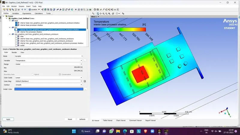
Temperature Contour:

CASE: 2: Refined Mesh

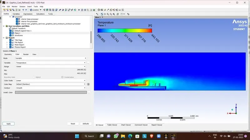
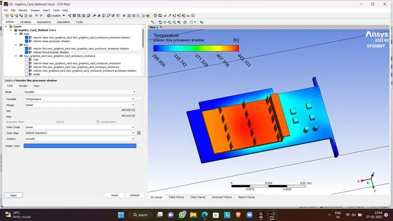
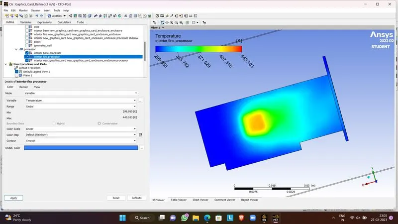
Inlet Velocity: 3 m/s.

RESIDUAL PLOT:

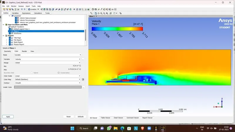
Velocity Contour:

Temperature Plot:

CASE 3: Refined Mesh

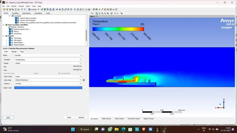
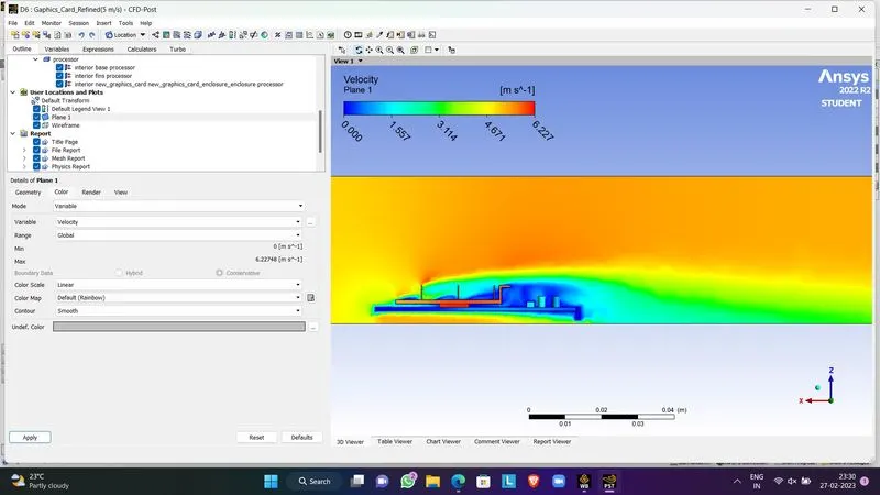
Inlet Velocity: 5 m/s

Residual Plot:

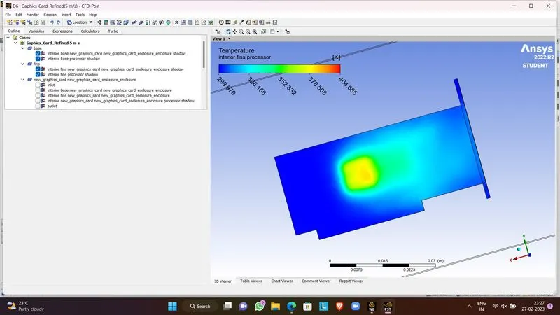
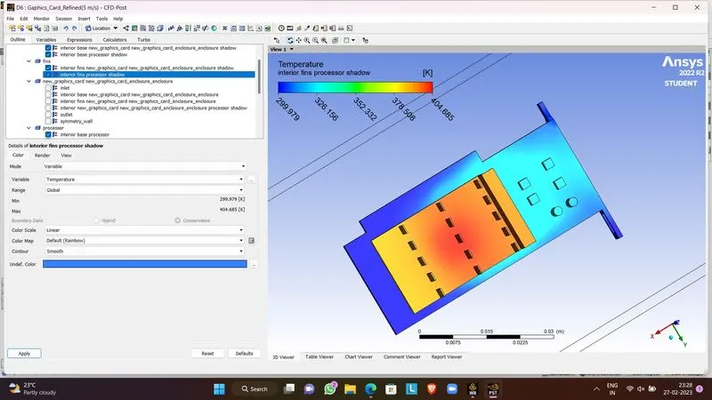
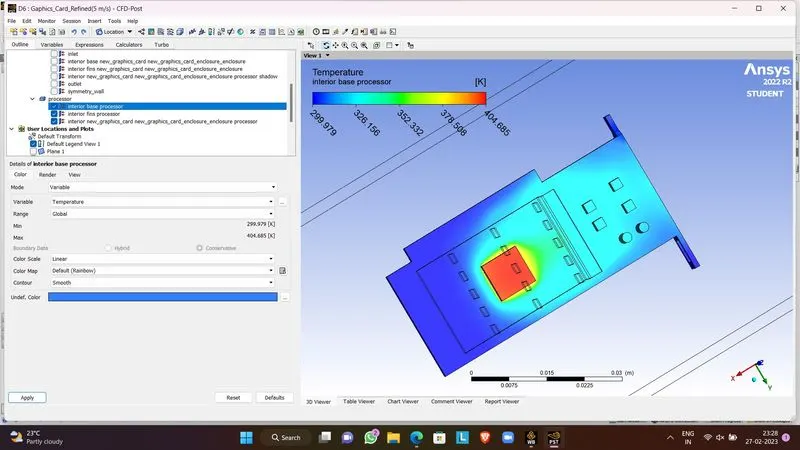
Temperature Plot:

Velocity Contour:

Observation:

SL NO.	Inlet Velocity	Maximum temperature at processor
1.	1 m/s (BaseLine Mesh)	593 K
2.	1 m/s (Refined Mesh)	594 K
3.	3 m/s (Refined Mesh)	443 K
4.	5 m/s (Refined Mesh)	404 K

Conclusion:

1. As the number of elements increases the accurate results of temperature distribution is obtained
2. From the above table, it is noted that the net temperature of components of graphics cards decreases with an increase in inlet velocity.
3. Higher inlet velocity results in better cooling and lower average temperature thus keeping the components safe from damage.