Week 3 - Solving second order ODEs

OBJECTIVE: Write a program to Simulate the transient behaviour of a Simple pendulum and create an Animation of it.

THEORY:

A Simple pendulum is an example of a Damped Simple Harmonic Motion. In this case, the motion of the Oscillator decreases with time and ultimately rest. This is called Damped motion. The motion works on the principle of Newton’s second law.

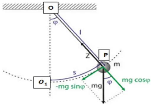
On Solving, We get a Ordinary Differential equation of 2^nd Order that describes the position of the ball with respect to time. The equation is given below:

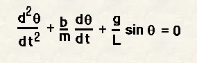
In this Equation:

b= Damping Coefficient, i.e. 0.05

m= mass of the bob i.e. 1 kg

L= Length of the string i.e. 1 m

g= Acceleration due to gravity i.e. 9.8 m/s^2

We need to convert the above given 2^nd order ODE to two 1^st order ODE and simulate the motion.

CODE:

% program to simulate and create an animation of a Simple Pendullum.
clear all
close all 
clc
% Input of Damping Coefficient
b = 0.05;
% Input of Acceleration due to gravity
g = 9.81;
%Length of String
l = 1;
% mass of bob
m = 1;

% initial condition
theta_0 = [0;3];

% time points
t_span = linspace(0,20,300);

% solve ODE 
[t,results] = ode45(@(t,theta) ode_func(t,theta,b,g,l,m),t_span,theta_0);

% Plot the graph for Time vs Displacement & Velocity
figure(1)
plot(t,results(:,1))
hold on 
plot(t,results(:,2))
ylabel('Velocity(Red) & Displacement(Blue)')
xlabel('time')
hold off
ct=1;
for i=1:length(t)
    x0=0;
    y0=0;
    x1= l*sin(results(i,1));
    y1= -l*cos(results(i,1));
    x2=-1;
    y2=0;
    x3=1;
    y3=0;

    figure(2)
    plot([x0 x1],[y0 y1],'linewidth',3,'color','b')
    hold on 
    plot(x1,y1,'o','markersize',20,'markerfacecolor','r')
    plot([x2 x3],[y2 y3],'linewidth',2,'color','g')
    axis([-2 2 -2 2]);
    pause(0.01);
    % Initializing an array to store each frame of graphs
    M(ct)=getframe(gcf);
    hold off
    ct=ct+1;
end
% Generate an Animation
movie(M)
videofile= VideoWriter('Simple pendullum.avi','Uncompressed AVI');
open(videofile)
writeVideo(videofile,M)
close(videofile)

FUNCTION:

function [dtheta_dt] = ode_func(t,theta,b,g,l,m)
  
   theta1 = theta(1);
   theta2 = theta(2);
   dtheta1_dt = theta2;
   dtheta2_dt = -(b/m)*theta2 - (g/l)*sin(theta1);
   dtheta_dt  = [dtheta1_dt; dtheta2_dt];
end

EXPLANATION:

• Input of value given such as b,m,L,g.
• Create an array theta_0 to store the initial displacement as 0m/s and Initial velocity as 3 rad/sec
• Create an array to store time from 0 to 20 with 300 values in between.
• Solving the ODE by using an inbuilt Matlab function called ode45 which takes 2 input parameters as t and theta
• Defining another function as ode_func to solve the ODE by taking inputs of t, theta, b,g,L,m.
• Plot the graph for time vs Displacement and Velocity.
• A for loop is used to locate the position of the bob and for each position is stored in array M
• Stitching all the positions an animation is generated.

ERROR:

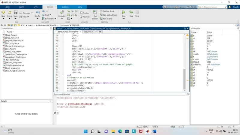
Wrong Command written to write the video file

OUTPUT:

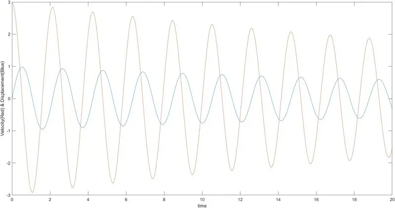
ANIMATION:

https://youtu.be/OvJkwBEf-GA