Week 4.1 - Genetic Algorithm
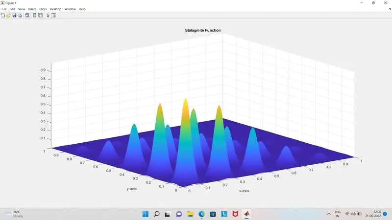
Aim: To optimise the stalagmite function and find the global maxima of the function.
THEORY:
Genetic Algoritm(GA) is a search based optimization technique based on concepts of evolutionary biology (Darwin’s theory of evolution) to find the global minima for optimization a problem. It is used to find the optimal or the near optimal solution to the given problems.It is generally used in research and in machine learning.
Optimization is a decision making process. It is a process where we put inputs in such a way that we get the "best" output for the problem. The definition of “best” varies from problem to problem, but in mathematical terms, it refers to maximizing or minimizing one or more objective functions, by varying the input parameters.
The Genetic algorithm uses the main types of rules at each step to create the new generation from the current population:
Initialization: Decide the population size or the set of data points from where we can select individuals and perform GA. If the size of population is more, we can get more accurate result.
Selection : Select the individuals, called parents that contribute to the population at the next generation. The fittest value will have the most probability to be selected.
Crossover: Combination of two parents to form children for the next generation
Mutation rules: Mutation occurs to maintain diversity within the population and prevent premature convergence . termination The algorithm terminates if the population has converged (does not produce offspring which are significantly different from the previous generation).
Fitness Function:The fitness function takes the solution as input and produces the suitability of the solution as the output. This evaluates how close the solution is to the optimal solution of the desired problem.
Syntax for genetic algorithm
x=ga(fun,nvars,A,B,Aeq,Beq, lb, ub,nonicon,Intcon.options)
This syntax is explained as follows:
‘x’ is the variable to store the output of the genetic algorithm.
‘fun’ is the function handle to call the function.
A and B are used to represent the linear inequalities of the function, if the linear inequalities do not exist, they can be empty set[].
Aeq and Beq are used to represent the equality constraints similarly, if the linear equalities do not exist, they can be empty set[].
‘ib' and 'ub are used to specify the upper and the lower bounds of the variables of the function.
‘nonlcon’ represents the non-linear constraints.
‘Intcon’ represents the integer constraint, such that the value of the function is an integer.
‘options’ used to provide the value of the default parameters used named parameters, if required to replace the default parameters. This is done by using the ‘optimoptions’.
STALAGMITE FUNCTION:
A stalagmite is a type of rock formation that rises from the floor of a cave due to the accumulation of material deposited on the floor from ceilings drippings.
A stalagmite function generally refers to the function with which we are generating values over a stalagmite kind of surface for finding out the local and global maxima and minima of that particular given function.
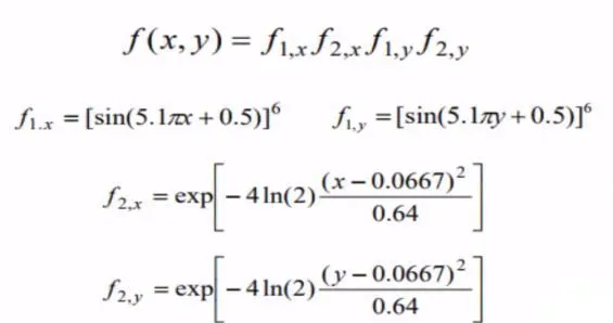
Given Function:
PROGRAM:
THE MAIN CODE:
% Maximization of a Stalagmite Function using Genetic Algorithm
clear all
close all
clc

% Defining the Inputs of the search space
x=linspace(0,1,150);
y=linspace(0,1,150);
num_spaces=50;

% Creating a 2-Dimensional Mesh
[xx,yy]= meshgrid(x,y);

% Nested loop for array value inputs
for i=1:length(xx)
    for j=1:length(yy)
        input_vector(1)=xx(i,j);
        input_vector(2)=yy(i,j);
        f(i,j)=get_stalagmite(input_vector);
    end
end

%plotting
figure(1)
surfc(xx,yy,-f);
shading interp
xlabel('x-axis')
ylabel('y-axis')
title('Stalagmite Function')

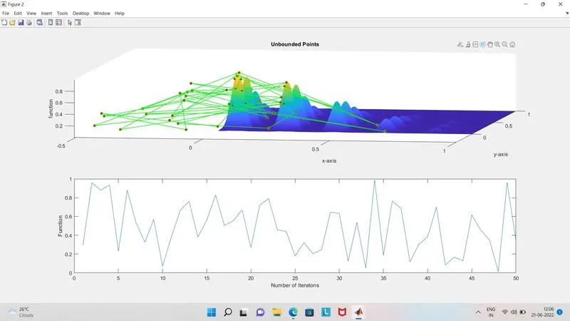
% Case:1 Statistical Behaviour of the Genetic Algoritm (Unbounded)

tic
for i=1:num_spaces
    [input1,fopt1(i)]=ga(@get_stalagmite,2);
    xopt1(i)=input1(1);
    yopt1(i)=input1(2);
end
Study_time1=toc;

%plotting
figure(2);
subplot(2,1,1);
hold on
surfc(xx,yy,-f);
xlabel('x-axis')
ylabel('y-axis')
zlabel('function')
shading interp;
plot3(xopt1,yopt1,-fopt1,'marker','o','markerfacecolor','r','markersize',5,'linewidth',1,'color','g');
title('Unbounded Points');
subplot(2,1,2);
plot(-fopt1);
xlabel('Number of Iteratons');
ylabel('Function');


%Case 2: Statistical Behaviour of Genetic Algorithm using Lower and Upper Bound

tic
for i=1:num_spaces
    [input2,fopt2(i)]=ga(@get_stalagmite,2,[],[],[],[],[0;0],[1;1]);
    xopt2(i)=input2(1);
    yopt2(i)=input2(2);
end
Study_time2=toc;

%plotting
figure(3)
subplot(2,1,1);
hold on
surfc(xx,yy,-f);
xlabel('x-axis')
ylabel('y-axis')
zlabel('function')
plot3(xopt2,yopt2,-fopt2,'marker','o','markerfacecolor','r','markersize',5,'linewidth',1,'color','g');
title('Bounded Points');
shading interp;
subplot(2,1,2);
plot(-fopt2);
xlabel('Number of Iteratons');
ylabel('Function');


% Case 3:Statistical behaviour of GA by increasing the number of iterations.

options=optimoptions('ga');
options=optimoptions(options,'PopulationSize',300);
tic
for i=1:num_spaces
    [input3,fopt3(i)]=ga(@get_stalagmite,2,[],[],[],[],[0,0],[1,1],[],[],options);
    xopt3(i)=input3(1);
    yopt3(i)=input3(2);
end
study_time3= toc;

%plotting
figure(4)
subplot(2,1,1);
hold on
surfc(xx,yy,-f);
xlabel('x-axis')
ylabel('y-axis')
zlabel('function')
shading interp;
plot3(xopt3,yopt3,-fopt3,'marker','o','markerfacecolor','r','markersize',5,'Linewidth',2,'color','g');
title('Bounded with Increased Population Size');
subplot(2,1,2);
plot(-fopt3);
xlabel('Number of Iterations');
ylabel('Functions');
EXPLANATION:
clear all
close all
clc
% Defining the Inputs of the search space
x=linspace(0,1,150);
y=linspace(0,1,150);
num_spaces=50;
% Creating a 2-Dimensional Mesh
[xx,yy]= meshgrid(x,y);
- In this part of the code we use the 'clear all', 'close all', 'clc' to clear all the previous plots, command window and the previous data.
- Defining two arrays x and y to store values from 0 to 1 storing 150 values in between them.
- Defining num_spaces for the GA operations to perform.
- Converting the two arrays into two 2-Dimensional arrays using 'meshgrid' command.
% Nested loop for array value inputs
for i=1:length(xx)
for j=1:length(yy)
input_vector(1)=xx(i,j);
input_vector(2)=yy(i,j);
f(i,j)=get_stalagmite(input_vector);
end
end
%plotting
figure(1)
surfc(xx,yy,-f);
shading interp
xlabel('x-axis')
ylabel('y-axis')
title('Stalagmite Function')
- In this part of the code, start a nested for loop starting from 1 to the length of the array.
- take each value of the array and store it an input_vector.
- Use a function get_stalagmite to calculate using the input_vector as argument and store in a array f.
- plot the stalagmite surface using surfc command
- For maximizing ,converting the values of the stalagmite function stored in the array f to their negative values. The minimum value of \'-f(x)\' is the maximum value of \'f(x).
OUTPUT:
% Case:1 Statistical Behaviour of the Genetic Algoritm (Unbounded)
tic
for i=1:num_spaces
[input1,fopt1(i)]=ga(@get_stalagmite,2);
xopt1(i)=input1(1);
yopt1(i)=input1(2);
end
Study_time1=toc;
%plotting
figure(2);
subplot(2,1,1);
hold on
surfc(xx,yy,-f);
xlabel('x-axis')
ylabel('y-axis')
zlabel('function')
shading interp;
plot3(xopt1,yopt1,-fopt1,'marker','o','markerfacecolor','r','markersize',5,'linewidth',1,'color','g');
title('Unbounded Points');
subplot(2,1,2);
plot(-fopt1);
xlabel('Number of Iteratons');
ylabel('Function');
- In this part , tic and toc command is used to store the time taken for the code to evaluate.
- num_spaces is used for the number of times the GA operations will be done.
- for every input stalagmite function will be evaluated and the value will stored in xopt1 and yopt1 respectively.
- The format of "ga" (genetic algorithm) used in this case is “[inputs, fopt] =ga (fun,nvars)”. Here inputs represent the values of the parameters x and y for which the function has the least value (fopt)”fun” is the function to be optimized, here it is a Stalagmite function, "nvars” the number of input variables, in this case its two “ input_vector(1)" and "input vector(2)”.
- Now for plotting the graph figure command is used for a new figure window, "subplot" is used for dividing the window in parts, and here it divides the figure window in two parts in the first two graphs are plotted in a single graph using the "hold” on command “surfc” command is used which plots a surface graph and the other graph is 3 dimensional line plot for this the command used is "plot3" X and Y label is given along with the title in the second half a ID plot is generated of values stored in "fopt1" using the plot command and then label the x-axis and y-axis.
OUTPUT:
%Case 2: Statistical Behaviour of Genetic Algorithm using Lower and Upper Bound
tic
for i=1:num_spaces
[input2,fopt2(i)]=ga(@get_stalagmite,2,[],[],[],[],[0;0],[1;1]);
xopt2(i)=input2(1);
yopt2(i)=input2(2);
end
Study_time2=toc;
%plotting
figure(3)
subplot(2,1,1);
hold on
surfc(xx,yy,-f);
xlabel('x-axis')
ylabel('y-axis')
zlabel('function')
plot3(xopt2,yopt2,-fopt2,'marker','o','markerfacecolor','r','markersize',5,'linewidth',1,'color','g');
title('Bounded Points');
shading interp;
subplot(2,1,2);
plot(-fopt2);
xlabel('Number of Iteratons');
ylabel('Function');
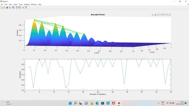
- In this part of the code we consider the upper and the lower bounds for the GA operations to perform. The numebr of iterations is 50 and stored in num_spaces and the tic and toc command is used to calculate the time taken for the code.
- The format of GA (genetic algorithm) used in this case is [inputs, fopt] = ga(fun,nvars A.b.Aeq.beq lb,ub) Here "inputs represents the values of the parameters x and y for which the function has the least value (fopt2) "fun" is the function to be optimized, here it is a Stalagmite function, "nvars in the number of input variables in this case its two, "input_vector(1)" and "input_vector(2) "A" is the linear inequality constraints real matrix, if there are none, then [],”b” is the linear inequality constraints real vector, if there are none, then []. "Aeq" is the linear inequality constraints real matrix, if there are none, then []; “beq" is the linear inequality constraints: real vector, if there are none, then [], "lb" is the lower bounds, specified as areal vector or array, "ub" is the upper bounds, specified as a real vector or array.
- Now for plotting the surface new figure is used and it is divided into two parts using subplot and the surface graph is plotted using surfc and the 3 dimensional line plot is plotted using plot3 command.label is given along with the title. Now in the second half a 1D plot is generated of values stored in “fopt2” using the “plot” command and then label the x-axis and y-axis.
- To maximize the stalagmite function '-' negative sign is used before fopt2.
OUTPUTS:
% Case 3:Statistical behaviour of GA by increasing the number of iterations.
options=optimoptions('ga');
options=optimoptions(options,'PopulationSize',300);
tic
for i=1:num_spaces
[input3,fopt3(i)]=ga(@get_stalagmite,2,[],[],[],[],[0,0],[1,1],[],[],options);
xopt3(i)=input3(1);
yopt3(i)=input3(2);
end
study_time3= toc;
%plotting
figure(4)
subplot(2,1,1);
hold on
surfc(xx,yy,-f);
xlabel('x-axis')
ylabel('y-axis')
zlabel('function')
shading interp;
plot3(xopt3,yopt3,-fopt3,'marker','o','markerfacecolor','r','markersize',5,'Linewidth',2,'color','g');
title('Bounded with Increased Population Size');
subplot(2,1,2);
plot(-fopt3);
xlabel('Number of Iterations');
ylabel('Functions');
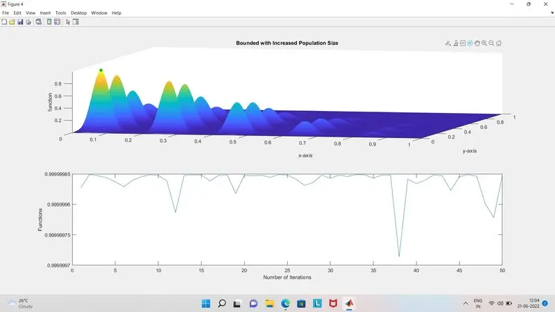
- In this part of the code, we see the statistical behaviour of the GA by increasing the number of Population size.The number of iterations a variable "num_cases” is used and is set to 50. For determining the time taken by then code to evaluate “tic and toc” command is used.
- The format of GA (genetic algorithm) used in this case is [inputs,fopt]=ga(fun,nvars,A,b,Aeq.beq.lb,ub.nonicon,intCon options)". Here inputs, fopt fun, nvars, A, b, Aeq, beq, lb and ub are same as mentioned as above,"nonicon” nonlinear constraints, specified as a function handle or function name, if there are none, then[], “intCon": integer variables, specified as a vector of positive integers, if there are none, then []. and "options" optimization options, specified as the out of optimizations or a structure.
- Now for plotting the graphs, "figure" command is used for a new figure window, subplot" is used for dividing the window in parts, and here it divides the figure window in two parts. In the first half two graphs are plotted a single graph using the "hold” on command, "surfc" command is used which flats a surface graph and the other graph is 3 dimensional line plot for this the command used is "plot3". X and Y label is given along with the title. Now in the second half 1D plot is generated of values stored in "fopt3” using the "plot" command and then label the x-axis and y-axis.
- a negative fopt3 is plotted in the graph as to find the global maxima from the stalagmite function.
OUTPUT:
FUNCTION CODE:
function f= get_stalagmite(input_vector)
a= input_vector(1);
b=input_vector(2);
f1_x= [sin((5.1*pi*a)+0.5)]^6;
f1_y= [sin((5.1*pi*b)+0.5)]^6;
f2_x = exp(-4*log(2)*(((a-0.0667)^2)/(0.64)));
f2_y = exp(-4*log(2)*(((b-0.0667)^2)/(0.64)));

f = -(f1_x*f1_y*f2_x*f2_y);
end
EXPLANATION:
- a Function named f is created and the input_vector is taken as arguments.
- each value of the input_vector is stored in each variable a and b.
- f is calculated using the variables and a negative sign is given to find the global maxima.
WORKSPACE:

ERRORS:
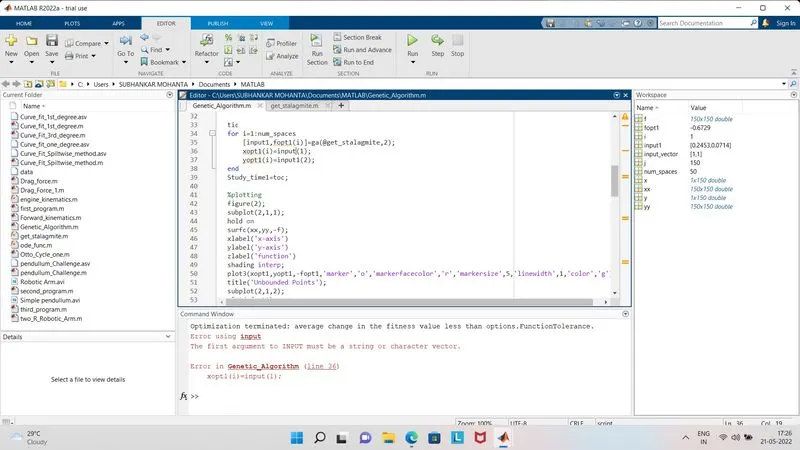
Wrong Variable name typed.
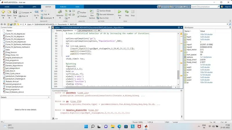
Wrong Number of Input Argument is typed. Wrong Syntax for GA operations
REFERENCES: