Week 3 - External flow simulation over an Ahmed body.

Aim: To perform external flow simulation over ahmed body for three cases of mesh from coarse to fine mesh and obtain the results of velocity contour, pressure contour and have a study of the wake region.

Introduction: Ahmed body is the reference body of the basic car model. It was orginally described by S.R Ahmed in 1984. The Ahmed body (Fig. 1) was first defined and its characteristics described in the experimental work of Ahmed [1]. Two configurations with slant angles of 25°and 35°are considered as a test case.In the experiment perform by the Ahmed [1], flow velocity was taken 60 m/s, Reynolds number was 4.29 million based on model length. This model is widely used in the research work and have plenty of results available for various parameters of flow velocity, slant angle difference in the model etc. The calculation of drag coefficient is given of utmost importance as it is dealt with the reduced flow consumption. Generally we will consider computational domain which is about 5 times of the length in the back region, while we will consider 2 times the length of the domain in the front region.

Theory: This is a case of external flow simulation. Here the air exerts pressure force normal to the surface and shear forces parallel to the surface along the surface of the body. The component of the resultant pressure and shear forces that act in the flow direction is called DRAG FORCE; the component that acts normal to the flow direction is LIFT FORCE. Mostly drag is an undesirable effect like friction and reduction of it is closely associated with reduction of fuel consumption in automobiles, submarines and aircraft; similarly improved safety and durability of structures subjected to high winds and reduction of noise and vibration. The drag is of two types: Pressure drag and friction drag. Generally two types of bodies are there: BLUNT and STREAMLINED. In blunt bodies pressure drag is dominant while friction drag is less while in streamlined bodies friction drag is dominant while pressure drag is less. In blunt body one way of reducing the pressure drag is by having the turbulence flow while in streamlined bodies one way of reducing friction drag is by delaying the turbulence flow and having laminar flow.

Solving and modelling approach: The ahmed body is imported into the Spaceclaim of Ansys Workbench. First we have to create enclosure of length 5m from back, 2m from the front, 1 m from top, 0 m from both and 0.5 m each from left and right of the ahmed body. The enclosure corresponds to the computational domain. Then we will see section mode and make sure no intereference is there and then we will enable share topology. make sure to suppress ahmed body. Then meshing is performed. First we start with the coarse mesh with base element size of 250 mm.; then in the legs of ahmed body face sizing of 5 mm is performed. Then in next case with element size of 100mm, face sizing of 3 mm; next case of 50 mm element size and 1 mm face sizing. We then check the mesh quality. Then we will give named selections of inlet, outlet, car wall and symmetry wall. Then we will open fluent solver. We enable pressure based with steady flow. Then in models we will enable K epsilon realizable enhanced wall treatment. Then we will give the inlet boundary condition of 25 m/sec and pressure outlet. Then the reference values are given; with area as projected area calculated from reports as 0.1315 m2 and length as 1.044 m. Then the solution is intialized. Then the report definitions are created for drag coefficient, lift coefficient. Then we will run for 350 iterations till solution converged. Then in post proceesor we will obtain necessary velocity and pressure contours by the creation of planes.

Preprocessing and solver settings.

(i) Geometry creation

First the geometry is imported into spaceclaim of ansys workbench of fluent. Then enclosures are created; and share topology is enabled. The enclosure dimension is 5 m from back, 2m from front, 1 m from top, 0 m from bottom and 0.5 m each from left and right.

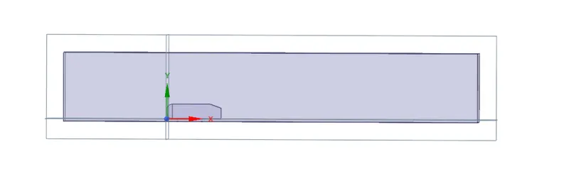
Fig 1 Geometry

(ii) Meshing

Then the meshing of the geometry is performed. First we do base mesh size of 250 mm. Then the face sizing of cylinder leg is done with 5 mm. The number of elements in first case is 85162 second case is 194100 and third case is 1080072 respectively.

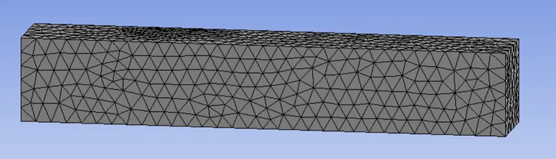
Fig 2 Meshing with base element size of 250mm

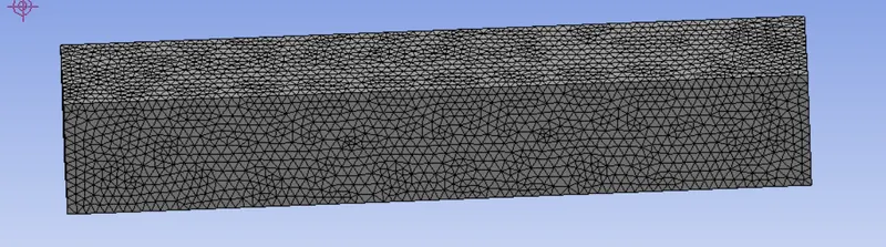
Fig 3 Meshing with base element size of 100mm

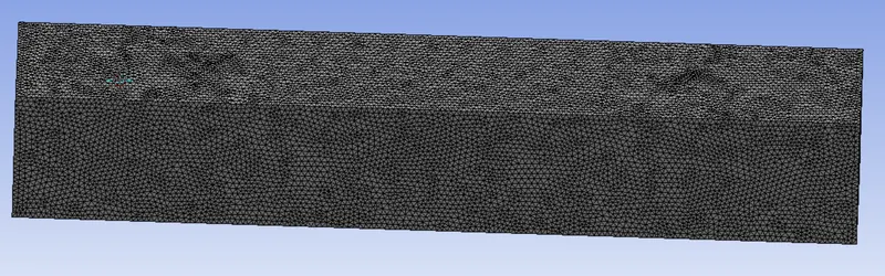
Fig 4 Meshing with base element size of 50mm

(iii) fluent solver proceesing

Now we will enable steady and pressure based solver.

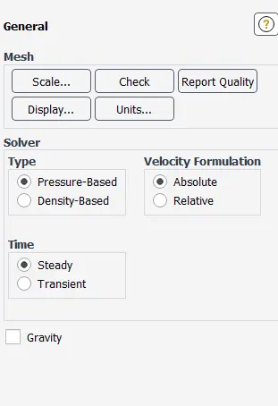
Fig 5 selecting pressure based solver

Then we will select the models. we go for k epsilon realizable enhanced wallt treatment model.

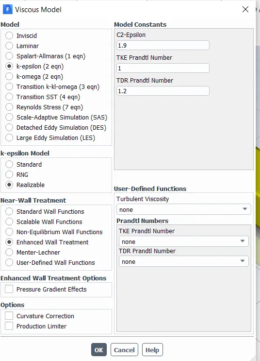
Fig 6 selecting model

Now we will give the boundary condition.

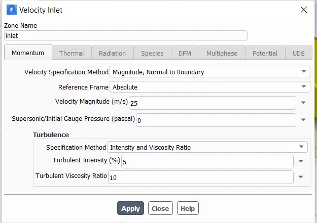
Fig 7 inlet boundary condition

We will give th einlet velocity of 25 m/sec .

For outlet we will give pressure outlet.

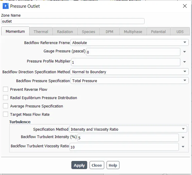
Fig 8 outlet boundary condition

Now we will give the reference values.

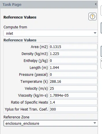
Fig 9 selecting reference values

The area is given as projected area and length is ahmed body length.

Now we will intialize the solution by hybrid intialization. Then we will create report definitions.

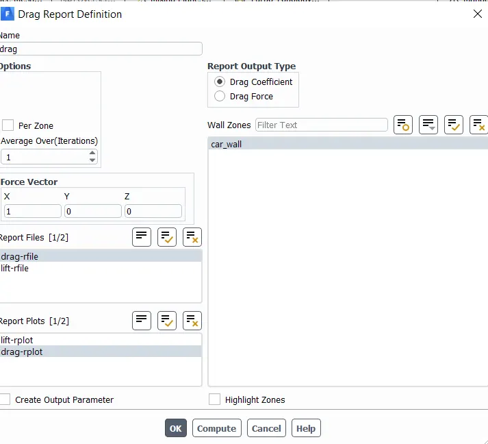
Fig 10 drag report file

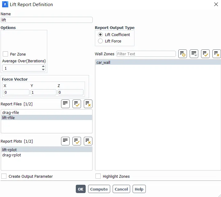
Fig 10 lift report file

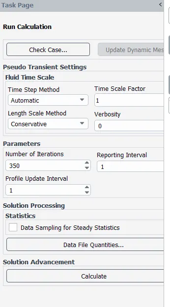
Fig 11 Run solution

Results

(i) Residual contours

(a) Base element size of 250mm

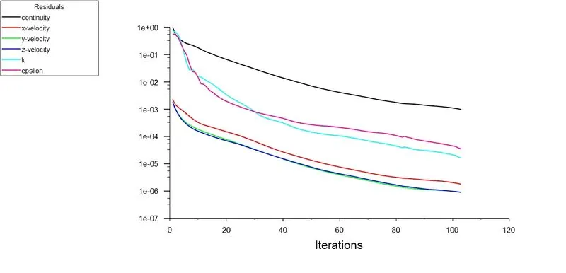
Fig 12 Residual contour for base element size of 250mm

(b) Base element size of 100 mm

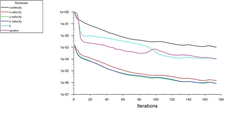
Fig 13 Residual contour for base element size of 100mm

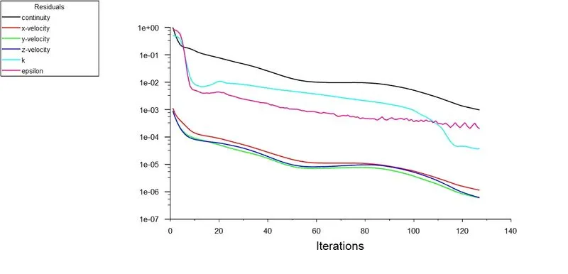
Fig 14 Residual contour for base element size of 50mm

The solution is run for 350 iterations, but the solutions are converged around 100, 170 and 130 iterations respectively.

(ii) Coefficient of drag

(a) Base element size of 250mm

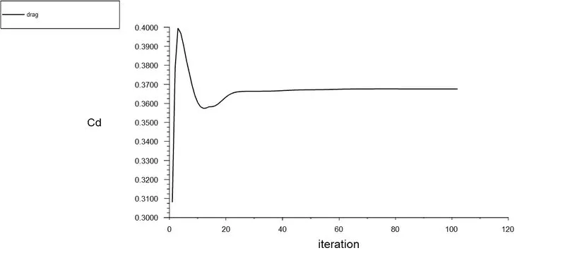
Fig 15 coefficient of drag for base element size of 250 mm

(b) Base element size of 100mm.

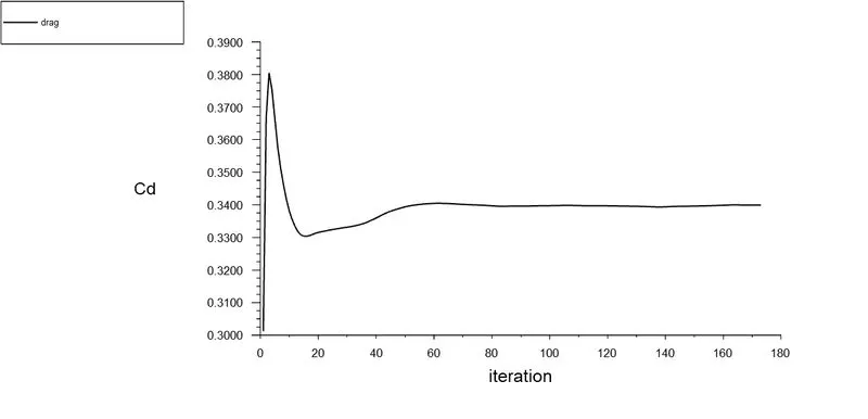
Fig 16 coefficient of drag for base element size of 100 mm

(b) Base element size of 50mm.

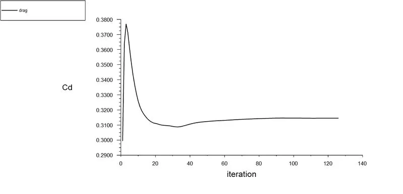
Fig 17 coefficient of drag for base element size of 50 mm

We can clearly see the coefficient of drag value decreases as the mesh is getting finer. We have Cd = 0.365 for a coarse mesh, while Cd = 0.315 as the mesh is getting finer.

(iii) Coefficient of lift

(a) Base element size of 250mm.

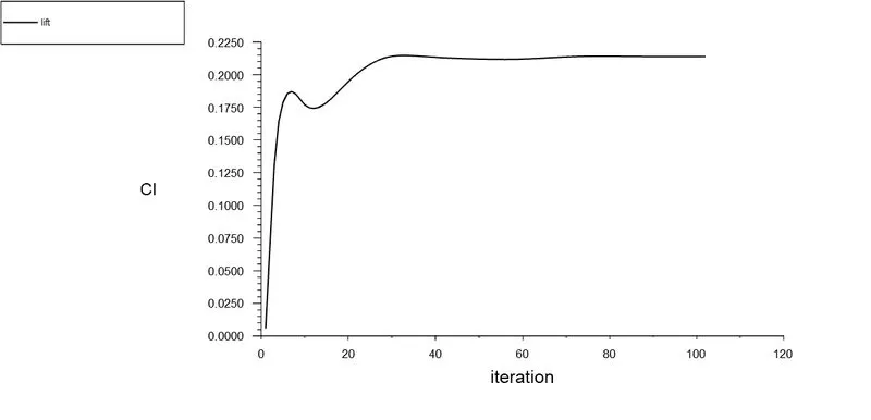
Fig 18 coefficient of lift for base element size of 250 mm

(b) Base element size of 100mm.

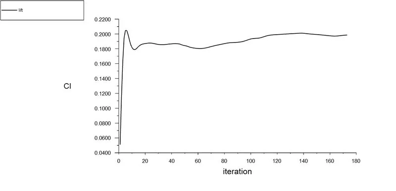
Fig 19 coefficient of lift for base element size of 100 mm

(c) Base element size of 50mm.

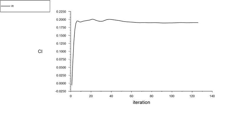
Fig 20 coefficient of lift for base element size of 50 mm

(iv) Velocity contour

(a) Base element size of 250mm.

\

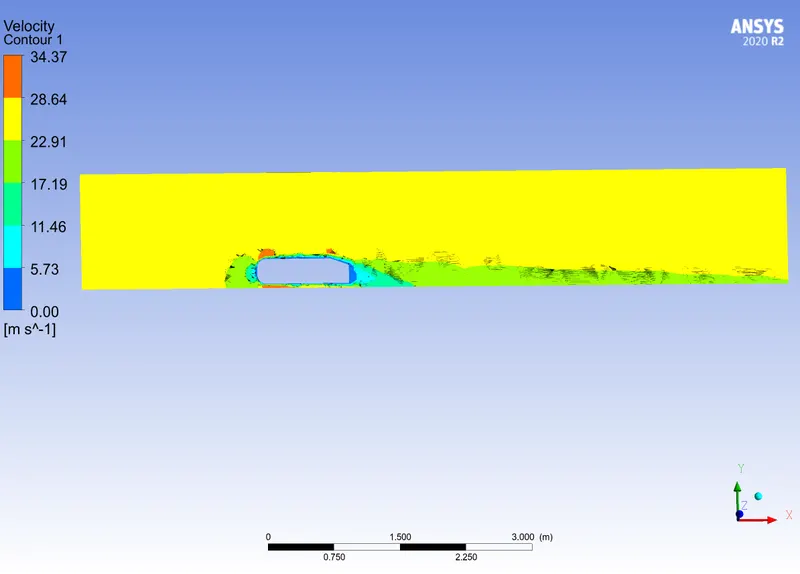Fig 21 Velocity contour for base element size of 250mm

We can see the velocity contour plot. Here velocity is zero at the starting point because of obstruction hence static pressure will be high. We can clearly see the velocity of air gets decreased in the vicinity of the ahmed body because of the boundary layer effect.

(b) Base element size of 100mm.

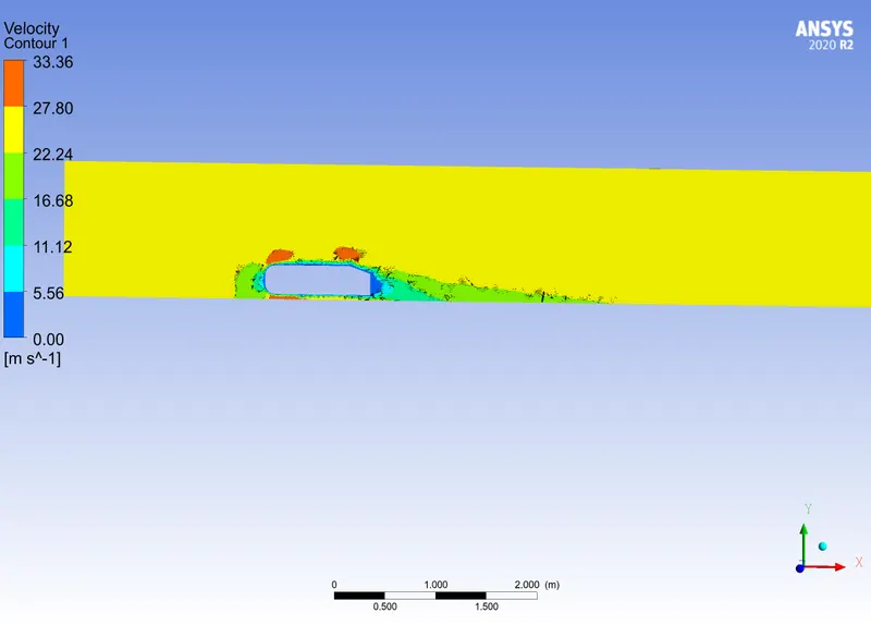
Fig 22 Velocity contour for base element size of 100mm

We can clearly see that since the mesh is finer than above case we can observe better velocity distribution here,

c) Base element size of 50mm.

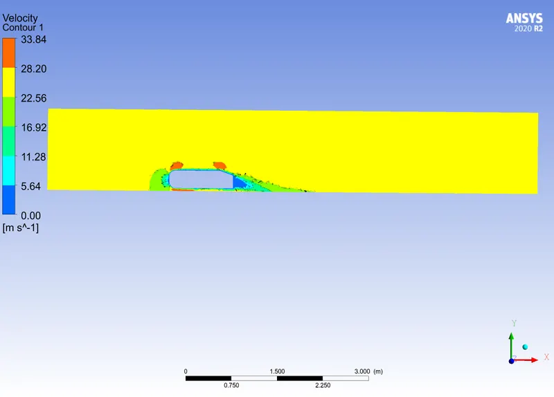
Fig 23 Velocity contour for base element size of 50mm

(v) Pressure contour

(a) Base element size of 250mm.

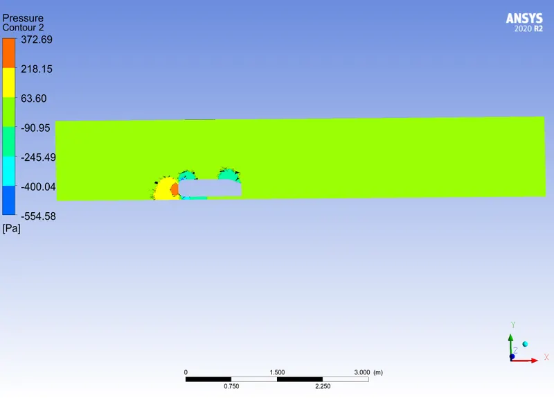
Fig 24 pressure contour for base element size of 250mm

(b) Base element size of 100mm.

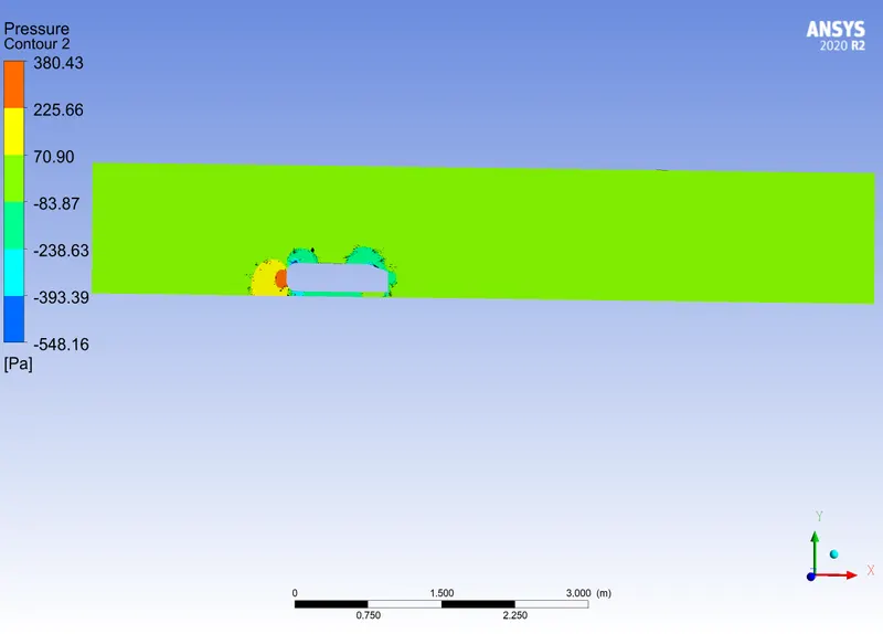
Fig 25 pressure contour for base element size of 100mm

(c) Base element size of 50 mm.

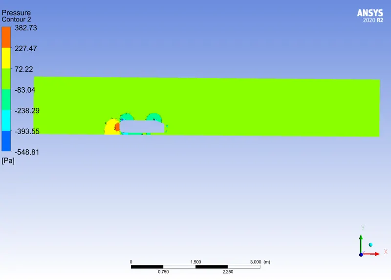
Fig 25 pressure contour for base element size of 100mm

The static pressure remains higher at the starting point, where velocity remains zero. Then the static pressure falls negative near the back side of the ahmed body.

(vi) Velocity vector contour

(a) Base element size of 250mm.

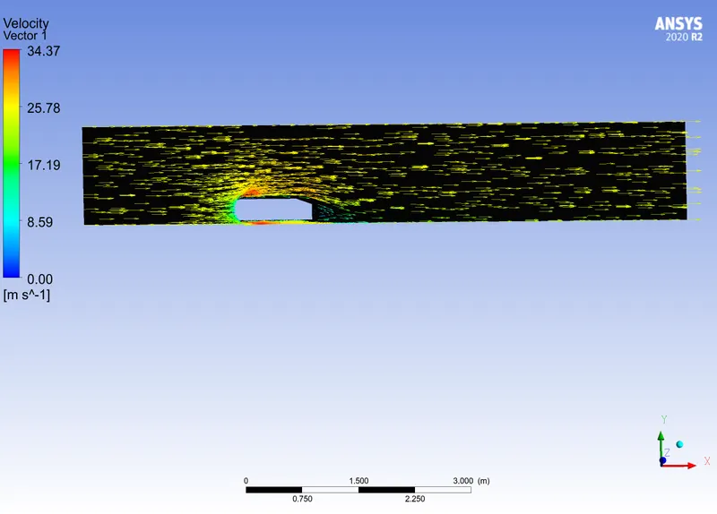
Fig 26 velocity vector contour for base element size of 250mm

(b) Base element size of 100mm.

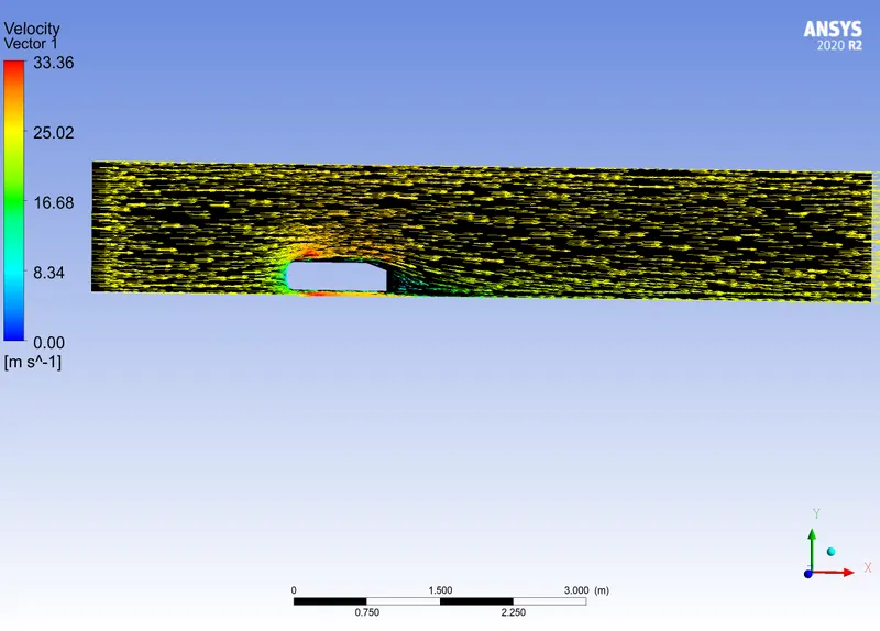
Fig 27 velocity vector contour for base element size of 100 mm

(c) Base element size of 50 mm.

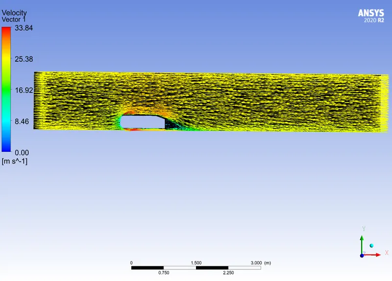
Fig 28 velocity vector contour for base element size of 50 mm

It is clearly observed that the velocity vector is clearly visible when the mesh is finer. We can also see the wake region beside the back side of the model, where slight backflow is observed.

Conclusions:

The simulation of ahmed body is performed for three mesh element sizes, from caorser to finer, with element size of 250 mm, 100mm and 50 mm. The number of elements obtained are 85162, 194100 and 1080072 respectively. We have obtained various contours like pressure contour , velocity contour, velocity vector contour then drag and lift coefficient report plots.

• The coefficient of drag obtained for element size of 250 mm is 0.4, while element size of 100mm is 0.38 while for element size of 50 mm is 0.375.
• The wake region is formed at the back side of the ahmed body. It is visible in the velocity vector plot, its clearly observed in the finer element size of 50mm.
• The stagnation point is clearly obtained in the contour where velocity is zero and pressure is maximum.