Week 6 - CHT Analysis on a Graphics card

Challenge 6 – Conjugate Heat Transfer Analysis on a Graphics Card

Aim – To conduct a conjugate heat transfer analysis on a graphics card and analyse the overall temperature of the components and the heat transfer coefficient of the processor

Solving and Modelling Approach –

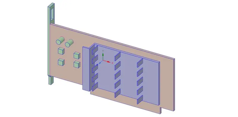
1. Firstly, the step file of the entire graphics card was imported into Spaceclaim.
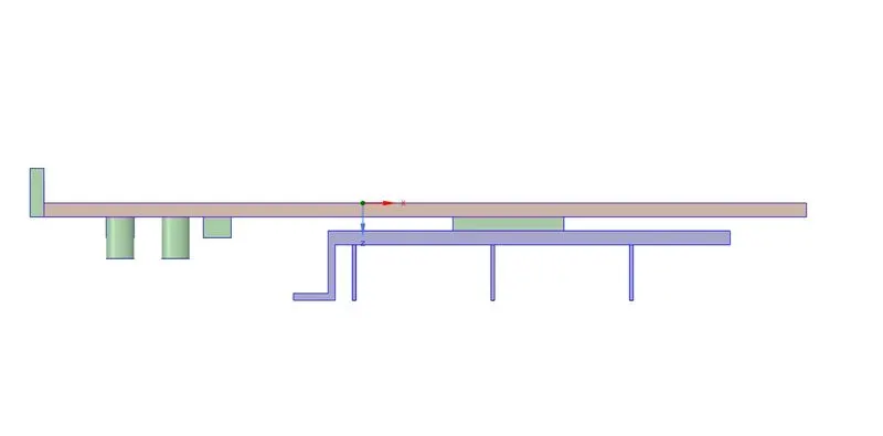
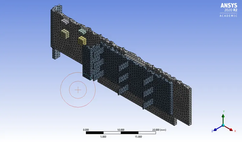
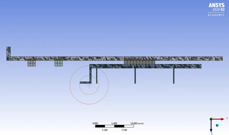
2. The graphics card consists of a processor, base and fins as 3 major components.
3. As the graphics card runs, it generates heat that can considerably damage other components in the vicinity due to high temperatures.
4. The fins of the graphics card is designed to increase the surface area for heat transfer thereby resulting in a lowered average temperature.
5. For this particular simulation, the base, processor, and fins were considered as solid bodies.
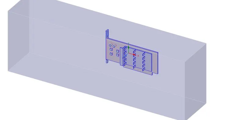
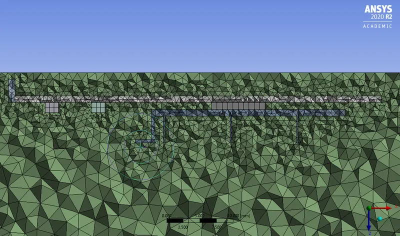
6. An enclosure, as shown below, was created around the graphics card for simulation purposes.
7. One end of the enclosure will be considered as an inlet for air to flow on the graphics card, thus cooling the overall component.
8. To obtain a conformal mesh between the solid and fluid boundaries, “share topology” option was enabled to share.
9. The model was then imported into the mesh interface for mesh generation

Meshing –

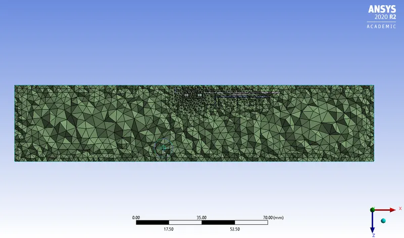
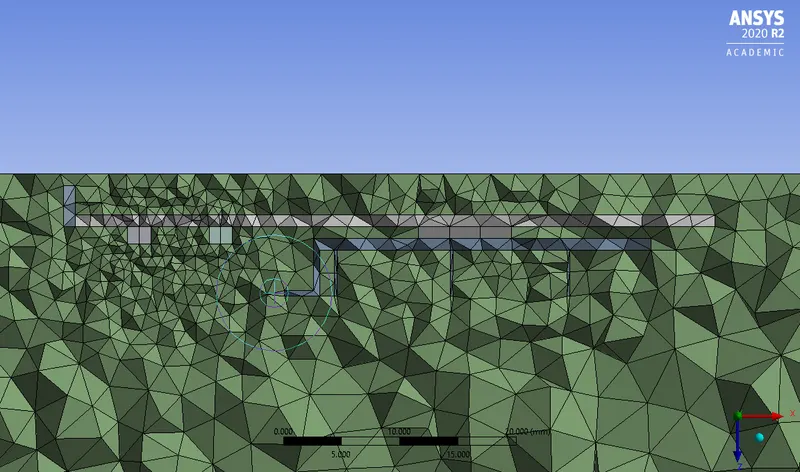
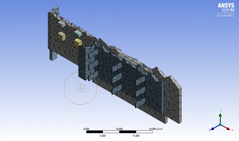
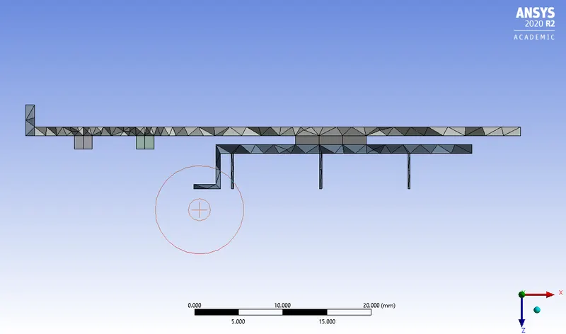
3 different mesh sizes were studied under this project as follows.

1. Baseline mesh – size = 5mm --- total mesh count = 212,000

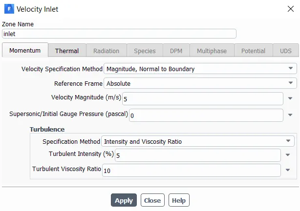
• Inlet velocity = 5m/s
• A baseline mesh was created and simulated for checking whether the simulation runs properly without any errors.

2. Medium Refined Mesh --- total mesh count = 318,000

• Overall global mesh size = 5mm
• Body sizing of fins = 0.8mm
• Body sizing of processor = 0.8mm
• Body sizing of base = 0.8mm
• Body sizing of enclosure = 3.5mm

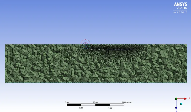
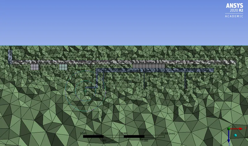
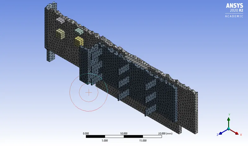
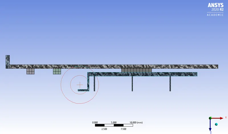
3. Highly Refined Mesh --- total mesh count = 490,000

• Overall global mesh size = 5mm
• Body sizing of fins = 0.8mm
• Body sizing of processor = 0.8mm
• Body sizing of base = 0.8mm
• Body sizing of enclosure = 2.5mm
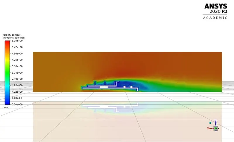
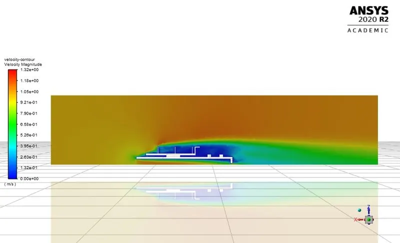
• The highly refined mesh was analysed for an inlet velocity of 1, 3, and 5m/s to analyse the effect of the air velocity on cooling and final temperature distribution.
• Afterwards the named selections were created
• The lateral face closer to the graphics card was named as an inlet, and the opposite face was chosen as a pressure outlet.
• All other faces were chosen as a symmetry
• Moreover, the processor, base and fins were chosen using box select and named accordingly.

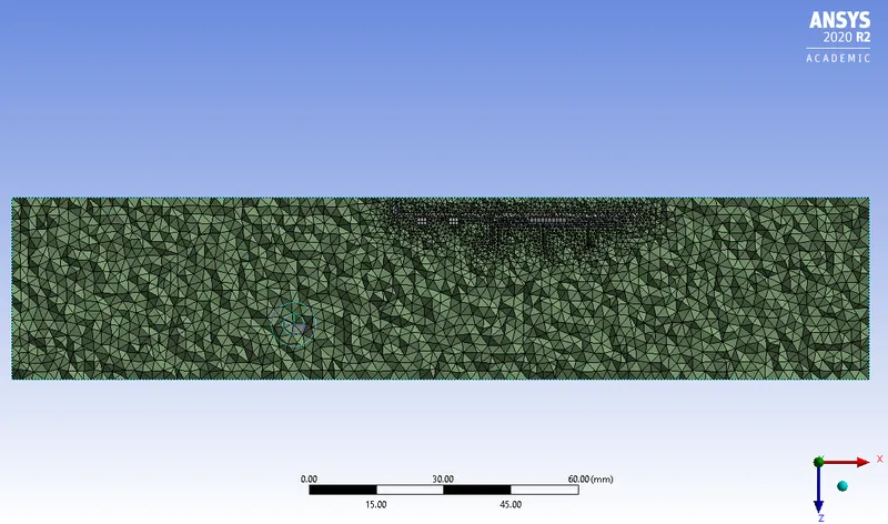
Setting up the case in Ansys Setup –

1. Since the velocities considered for this particular problem are 1, 3, and 5m/s which is very small as compared to the velocity of sound, the Mach number is <<< 0.3.
2. Hence, a pressure-based solver was used since there are low chances of compression.
3. The problem was analysed in a steady state manner since we are only analysing the end results
4. Since this problem statement requires to calculate the wall heat transfer coefficient, a K-omega SST viscous turbulence model was used since this model is more accurate at capturing wall effects as compared to other models such as the k-epsilon model.
5. Then, materials were added for the solid domains.
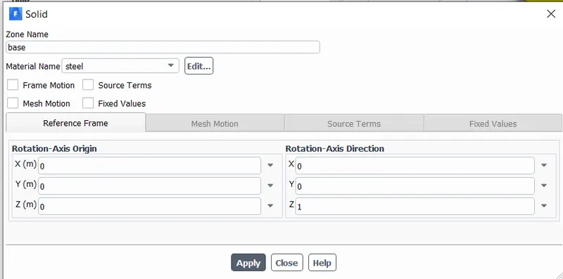
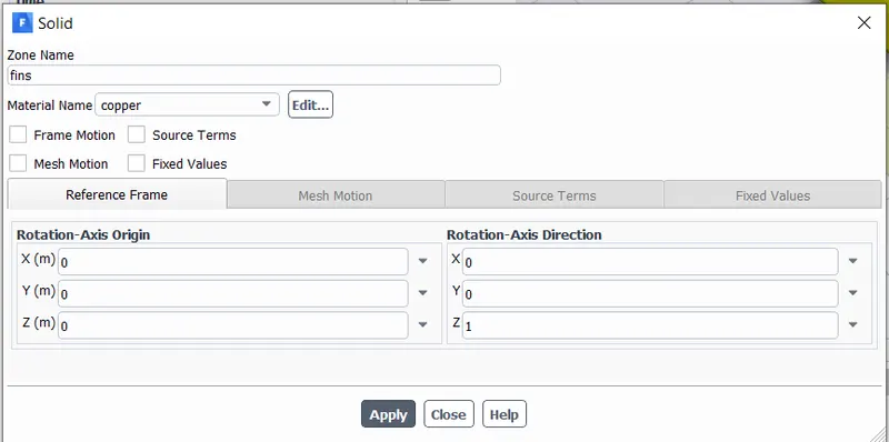
6. Steel, copper, and silicon were used for the base, fins, and processor respectively.
7. The materials for each component were taken from several articles from the internet.
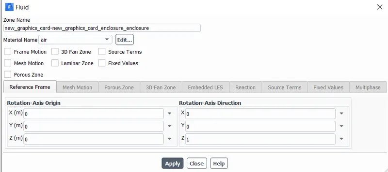
8. Afterwards, all the domains were assigned to either solid or fluid in the cell zone conditions, the enclosure being the only fluid domain, and the components represented the solid domains.
9. The respective material for each component was added in the cell zone conditions.
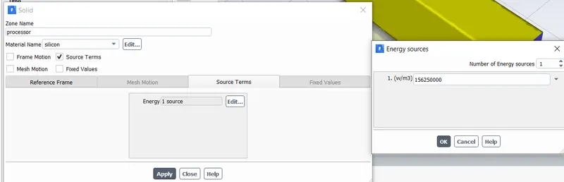
10. Since this problem involves the processor being a source of heat generation, an energy source term was applied to the processor domain
11. The processor is component which exists between the base and fins.
12. As the usage increases, the processor produces heat and the base is used to support the overall assembly.
13. Let the thermal design power of the processor be considered as 10W from various sources on the net.
14. Next the volume of the processor is calculated
15. Heat generated by the processor = Power (W)/Volume of the processor = 10/64e-9

= 1.5625e8 W/m^3

16. The above value was inserted as a single source term of energy in the cell zone conditions of the processor
17. For boundary conditions, the velocity inlet value was given as per iteration and the outlet was considered as a pressure outlet.
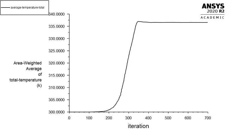
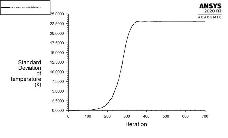
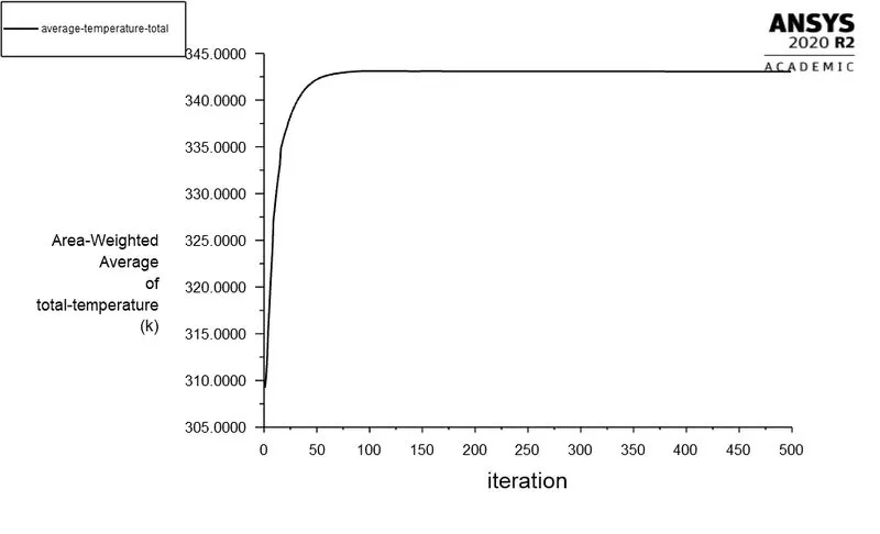
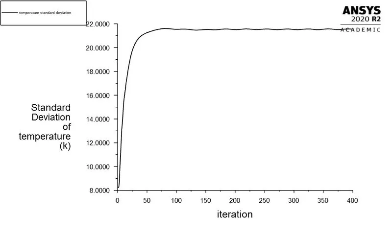
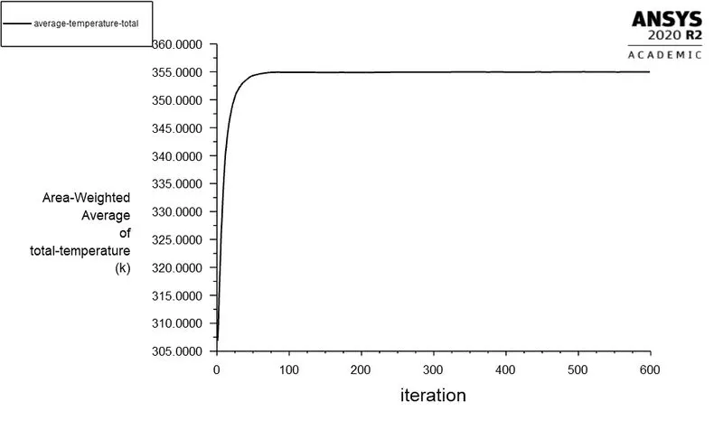
18. Afterwards, report definitions of standard deviation and area weighted average temperature of the 3 components was plotted while the simulation was running
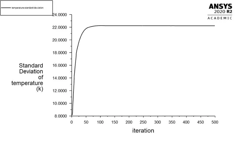
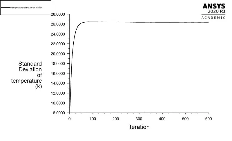
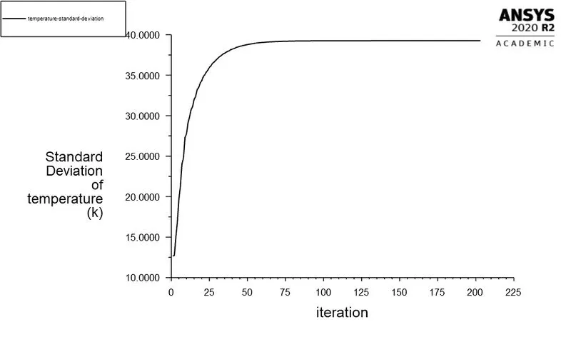
19. Standard deviation helps us identify whether the resultant temperature is fairly uniform or not, thereby giving an idea on the cooling effect.
20. Average temperature helps us understand the max and min temperature reached throughout the cooling process.
21. If the average temperature is low, this indicates that cooling has been successful
22. Furthermore, the solution was initialised using hybrid initialisation.
23. Velocity, pressure and temperature contours were plotted on a sample cut reference plane and observed using solution animations
24. A 3D contour of static and total temperature were also observed by creating solution animations.
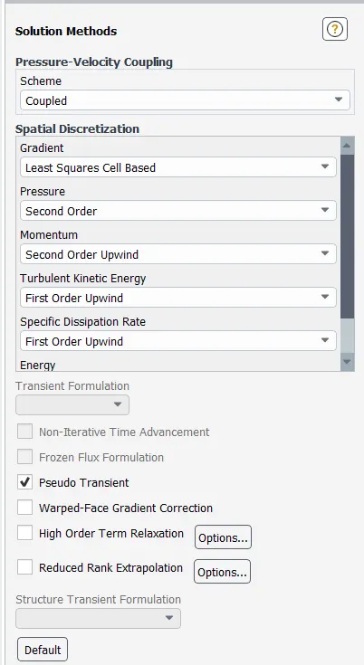
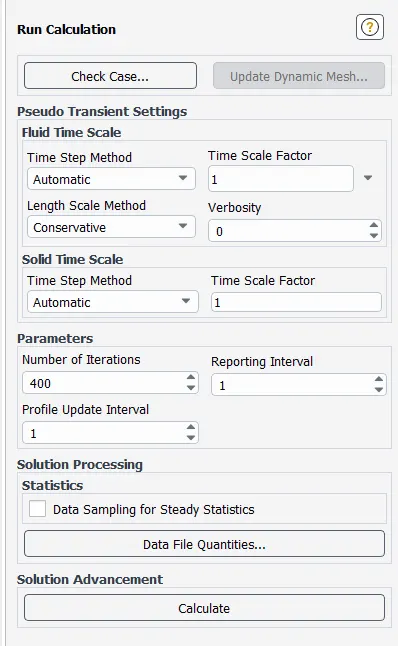
25. A coupled solution scheme was used and the solution was run for around 500 iterations.
26. After the simulations completed, the results were post processed

ENCLOSURE DOMAIN - AIR

BASE - STEEL

FINS - COPPER

PROCESSOR - SILICON - HEAT GENERATOR

Properties of solid and fluid zones –

Property/Material	air - enclosure	steel - base	copper - fins	silicon - processor
Density (kg/m^3)	1.225	8030	8978	2330
Specific heat at constant pressure (J/(kg⋅K))	1006.43	502.48	381	710
Thermal Conductivity (W/(m⋅K))	0.0242	16.27	387.6	150

Results –

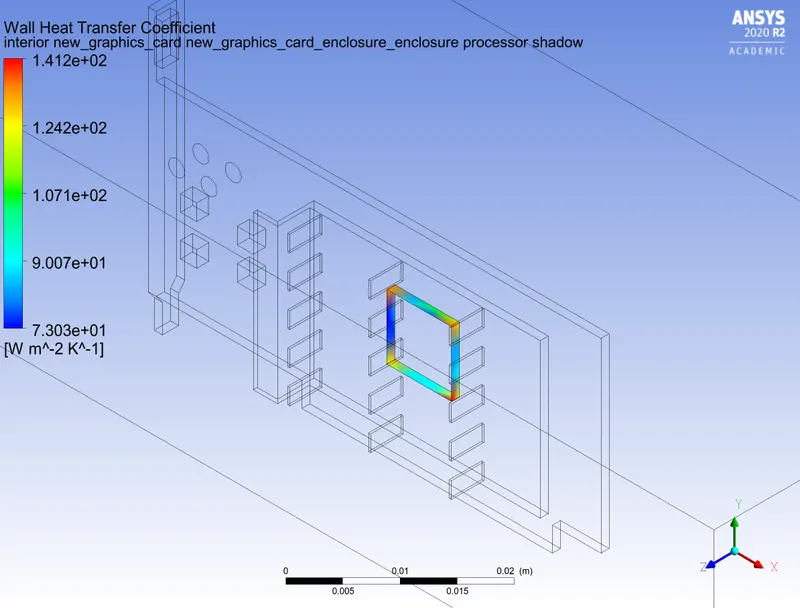
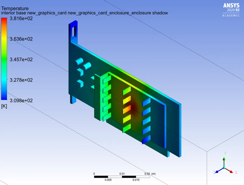
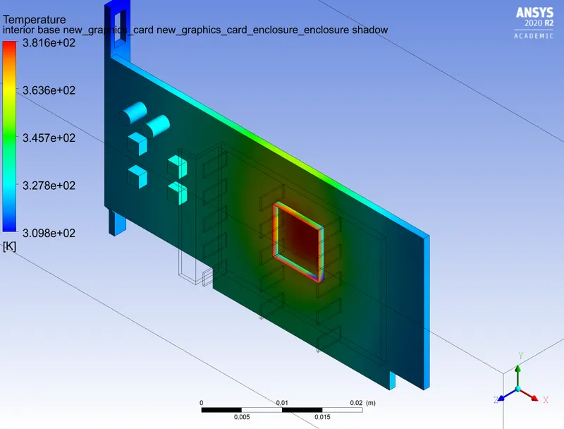
1. Baseline mesh – size = 5mm --- total mesh count = 212,000

• Inlet velocity = 5m/s
• A baseline mesh was created and simulated for checking whether the simulation runs properly without any errors.

2. Medium Refined Mesh --- total mesh count = 318,000

• Inlet velocity = 5m/s
• Overall global mesh size = 5mm
• Body sizing of fins = 0.8mm
• Body sizing of processor = 0.8mm
• Body sizing of base = 0.8mm
• Body sizing of enclosure = 3.5mm

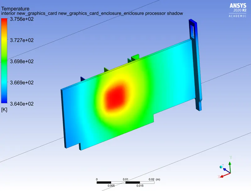
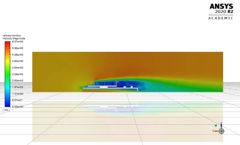
3. Highly Refined Mesh --- total mesh count = 490,000

• Inlet velocity = 5m/s
• Overall global mesh size = 5mm
• Body sizing of fins = 0.8mm
• Body sizing of processor = 0.8mm
• Body sizing of base = 0.8mm
• Body sizing of enclosure = 2.5mm

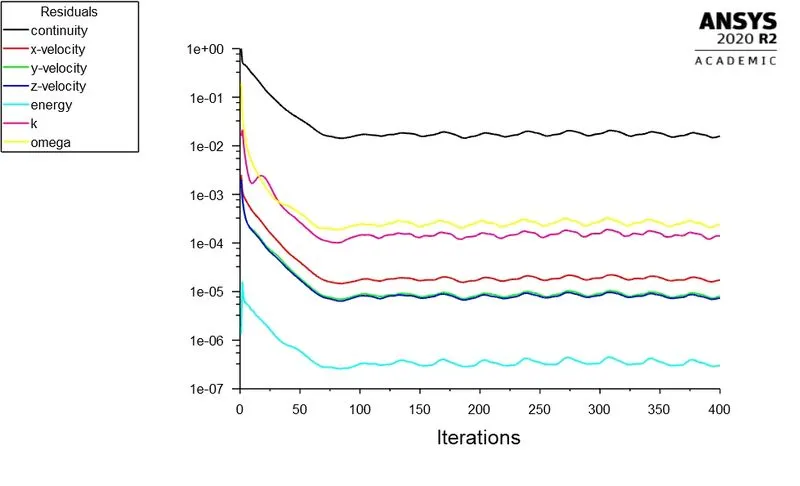
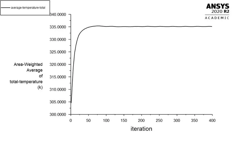
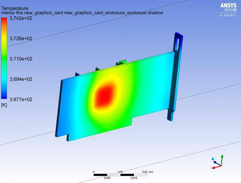
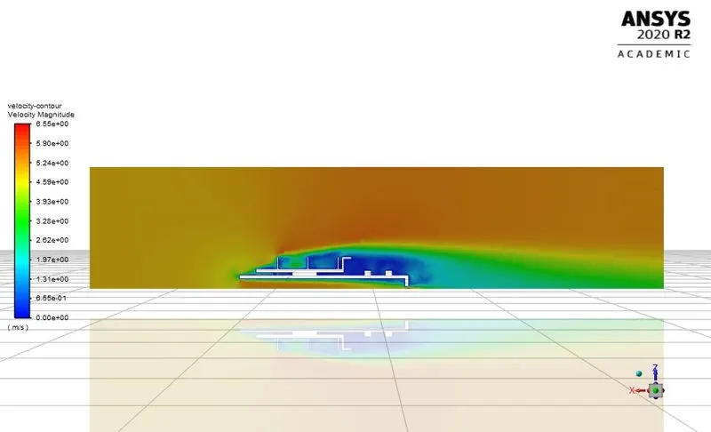
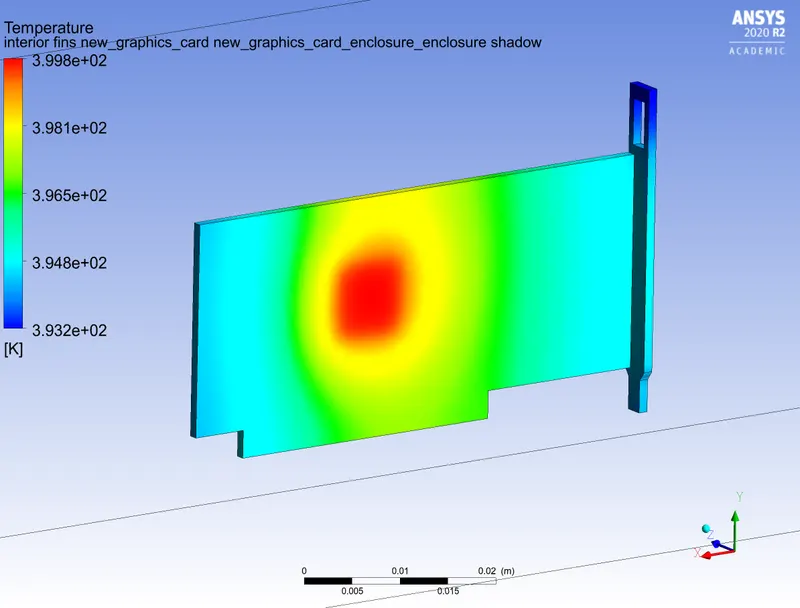
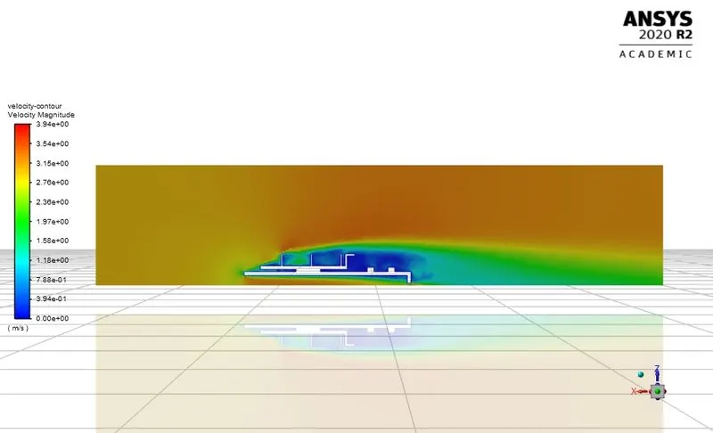
4. Highly Refined Mesh --- total mesh count = 490,000

• Inlet velocity = 3m/s
• Overall global mesh size = 5mm
• Body sizing of fins = 0.8mm
• Body sizing of processor = 0.8mm
• Body sizing of base = 0.8mm
• Body sizing of enclosure = 2.5mm

5. Highly Refined Mesh --- total mesh count = 490,000

• Inlet velocity = 1m/s
• Overall global mesh size = 5mm
• Body sizing of fins = 0.8mm
• Body sizing of processor = 0.8mm
• Body sizing of base = 0.8mm
• Body sizing of enclosure = 2.5mm

TABULAR OBSERVATIONS –

Iteration	Average temp (K)	Max Temp (K)	Wall HTC (W/(m2°K))	Standard Deviation Temp (K)
Baseline Mesh v = 5m/s	337	381.6	141.2	23
Medium Refined Mesh v = 5m/s	343	375.6	238.8	22
Highly refined Mesh v = 5m/s	334	374.2	234.4	21.5
Highly refined Mesh v = 3m/s	355	399.4	234.5	26
Highly refined Mesh v = 1m/s	432	493.3	234.3	38

Proof that the solutions have reached convergence -

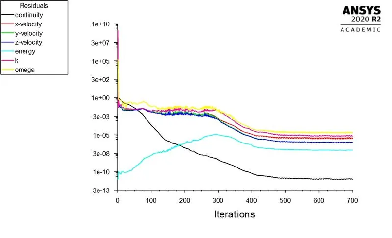
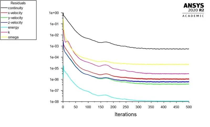
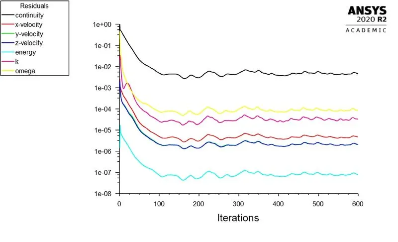
1. In the 1st iteration, it is clearly visible that the continutity, x-velocity, y-velocity, z-velocity, k and omega equations reach an absolute criteria of below 10^-3 - thus convergence has reached

2. In the 2nd iteration, it can be observed that equations start to oscillate after around 400 iterations, thus prooving that the solution has converged

3. In the 3rd iteration, it can be observed that equations start to oscillate after around 175 iterations, thus prooving that the solution has converged.

4. In the 4th iteration, it can be observed that equations start to oscillate after around 500 iterations, thus prooving that the solution has converged.

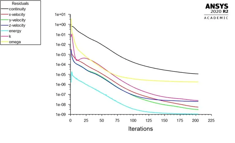
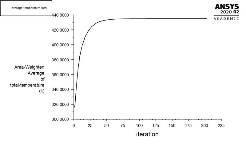
5. In the 5th iteration, it is clearly visible that the continutity, x-velocity, y-velocity, z-velocity, k and omega equations reach an absolute criteria of below 10^-3 after 200 iterations - thus convergence has reached

Potential Hotspots on the model

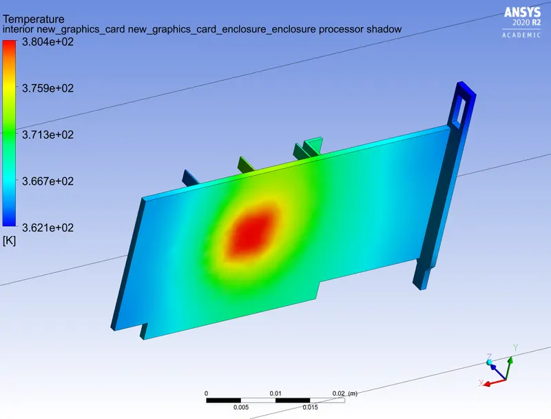
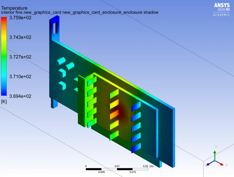
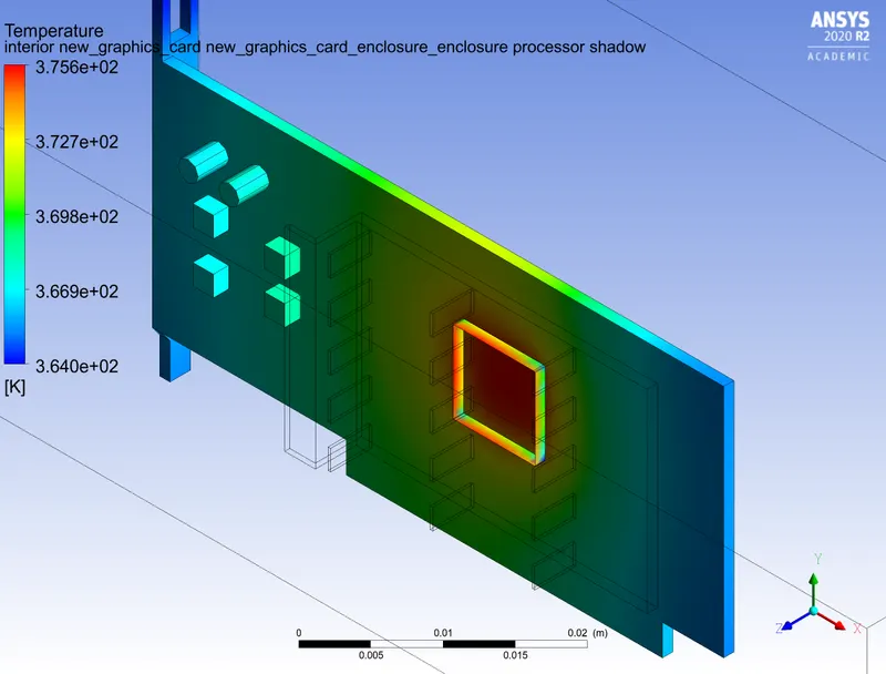
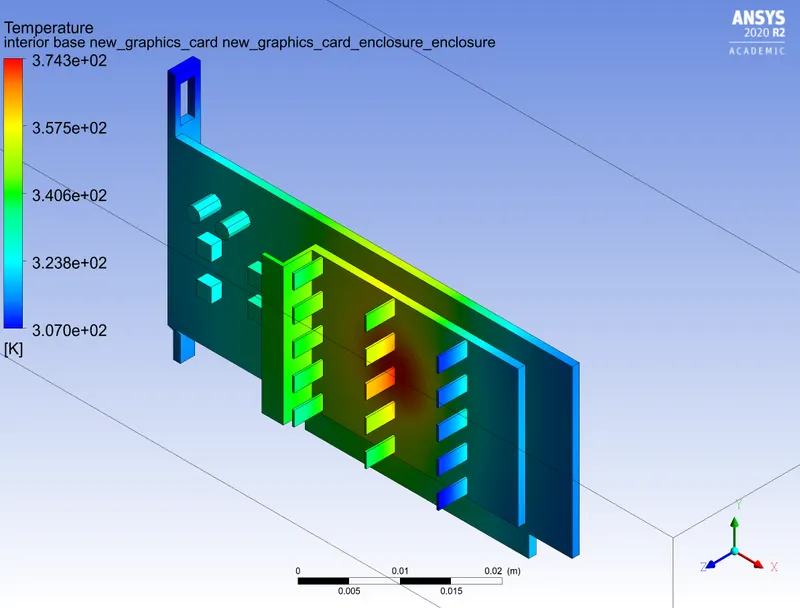
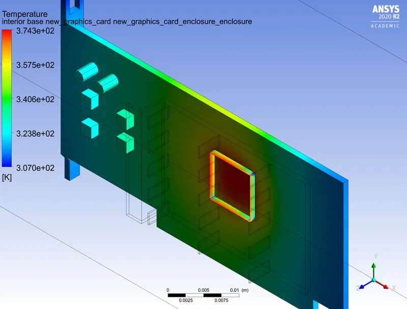
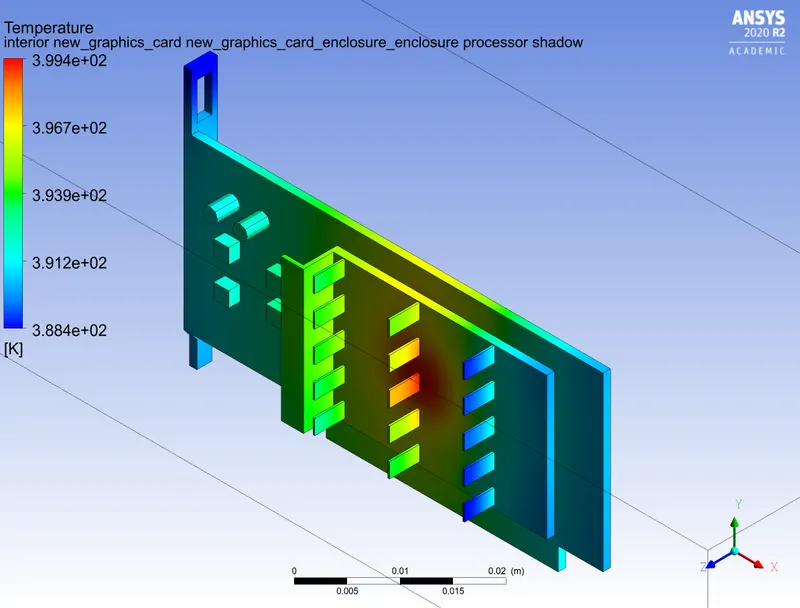
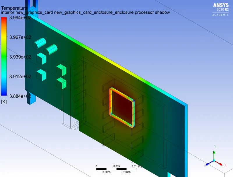
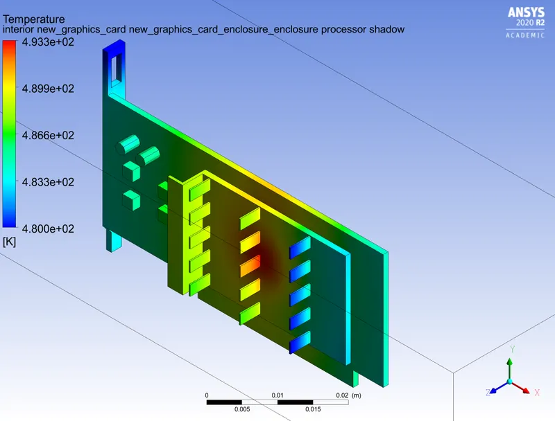
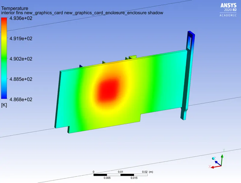
1. It can be observed that the fins that are closest to the processor have the maximum temperature on the surface. This is self explanatory since, those fins will accumulate more heat thus having a higher temperature.

2. The fins closest to the inlet velocity have lowest temperature since they are most away from the processor and they are cooled at a high velocity.

3. The fins farthest from the velocity inlet have an average temperature distribution.

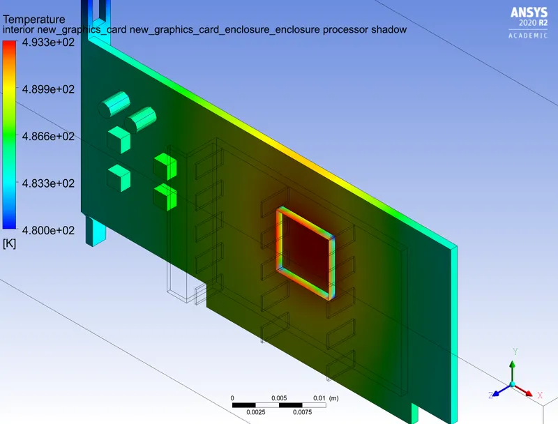
4. Concerning theh base, the temperature at a particular point increases as the distance between the point and processor becomes lesser. Hence the temperature on the base shows a smooth transition of temperature

CONCLUSIONS AND INFERENCES –

1. From the above table it is fairly notable that the net temperature of components of the graphics card decreases with increase in inlet velocity.
2. Hence, it can be inferred that a higher inlet velocity results in better cooling and lowering of the average temperature thus keeping the components safe from damage.
3. Furthermore, it can be observed that the max temperature increases significantly from 399 to 493 m/s when the inlet velocity is reduced from 3m/s to 1m/s, also proving that a high velocity is required for better cooling
4. When it comes to standard deviation of temperature of the components, the last iteration with an inlet velocity of 1m/s had the highest value of standard deviation.
5. This indicates that the temperature distribution becomes less uniform as the inlet velocity decreases
6. Iterations 1, 2, and 3 with an inlet velocity of 5m/s showed similar results of standard deviation around 22K.
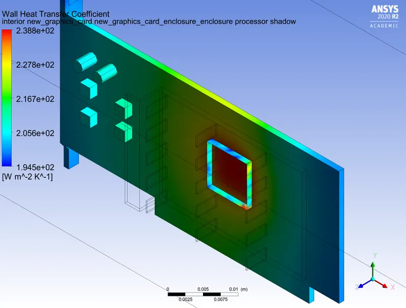
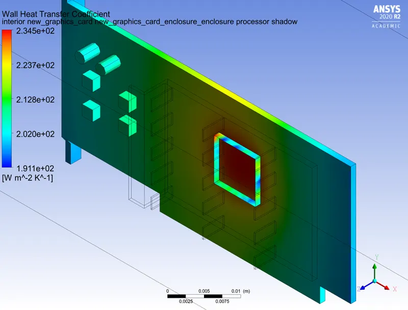
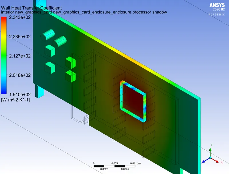
7. Wall heat transfer coefficient is one parameter which is highly dependent on mesh refinement.
8. Since wall heat transfer coefficient is calculated on the first mesh layer on the boundary, a finer mesh will yield more accurate and precise results
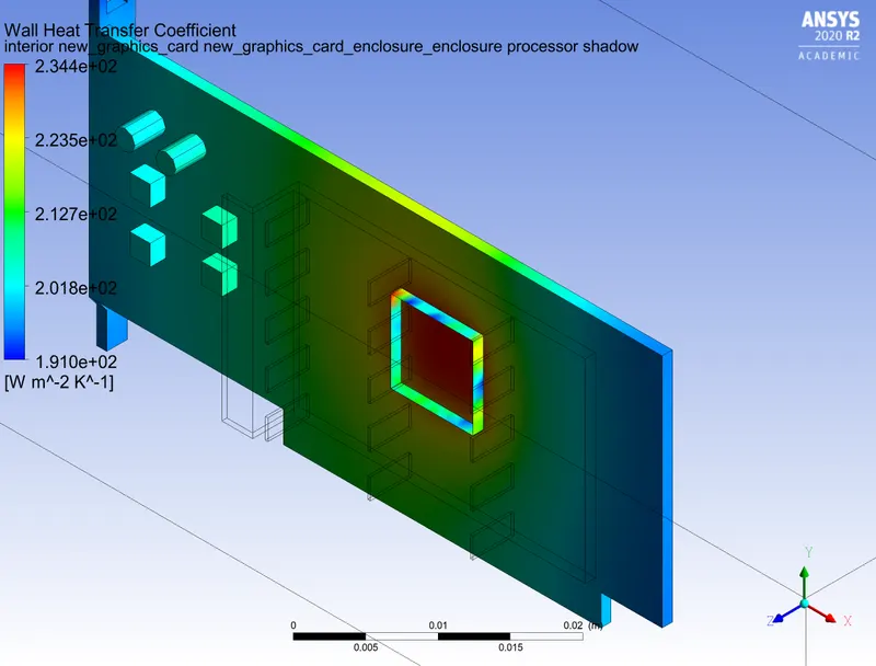
9. The 1^st iteration with a baseline mesh resulted in a wall HTC of 141.2 W/(m²°K), whereas all other iterations gave a wall HTC of around 235 W/(m²°K)
10. Hence 235 W/(m²°K) can be considered as an accurate wall heat transfer coefficient value