Week 5 - Rayleigh Taylor Instability

Challenge 5 – Rayleigh Taylor Instability

Aim – To study the Rayleigh Taylor Instability and explain the effects of mesh size on simulation results and time step size.

What are some practical CFD models that have been based on the mathematical analysis of Rayleigh Taylor waves?

1. Kelvin-Helmholtz Instability – The KH instability is a hydrodynamic instability in which immiscible, incompressible, and inviscid fluids are in relative and irrotational motion. In KHI, the velocity and density profiles are uniform in each fluid layer, but they are discontinuous at the (plane) interface between the two fluids. This discontinuity in the (tangential) velocity, i.e., the shear flow, induces vorticity at the interface; as a result, the interface becomes an unstable vortex sheet that rolls up into a spiral. KHI is observed in a wide range of nature. Examples are listed below

• Ocean mixing in meteorology 
• Motion of interstellar clouds 
• Clumping in supernova remnants
• Production of unstable shear layer and vortices in high energy density plasmas 

2. Plateau–Rayleigh instability - Often just called the Rayleigh instability, explains why and how a falling stream of fluid breaks up into smaller packets with the same volume but less surface area. It is related to the Rayleigh Taylor Instability and is part of a greater branch of fluid dynamics concerned with fluid thread breakup. This fluid instability is exploited in the design of a particular type of ink jet technology whereby a jet of liquid is perturbed into a steady stream of droplets. The driving force of the Plateau–Rayleigh instability is that liquids, by virtue of their surface tensions, tend to minimize their surface area. A considerable amount of work has been done recently on the final pinching profile by attacking it with self-similar solutions.
3. Richtmyer–Meshkov instability – The RM instability is the fluid flow phenomenon that occurs when a shock wave impinges (in the normal direction) upon an interface separating two gases having different densities. The instability causes perturbations on the interface to grow, producing vortical structures which potentially result in a turbulent mixing layer

Solving and Modelling Approach –

1. To understand the Rayleigh Taylor Instability phenomenon a 2D geometry has been taken into consideration.
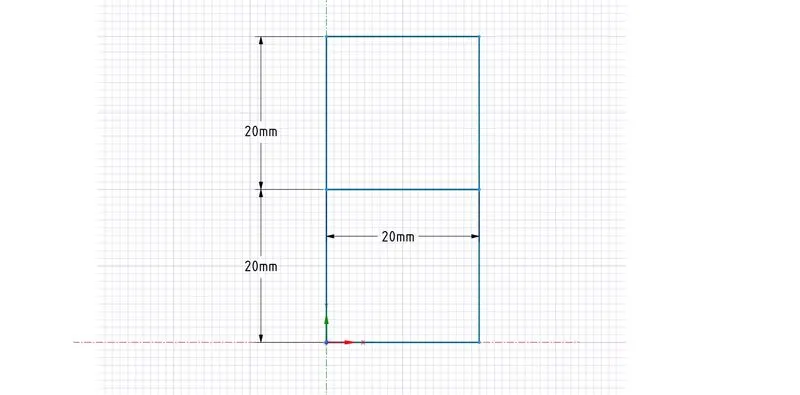
2. Two squares each of edge length 20mm were created on top of each other in Spaceclaim.
3. Using the pull feature, the squares were created into surface entities.
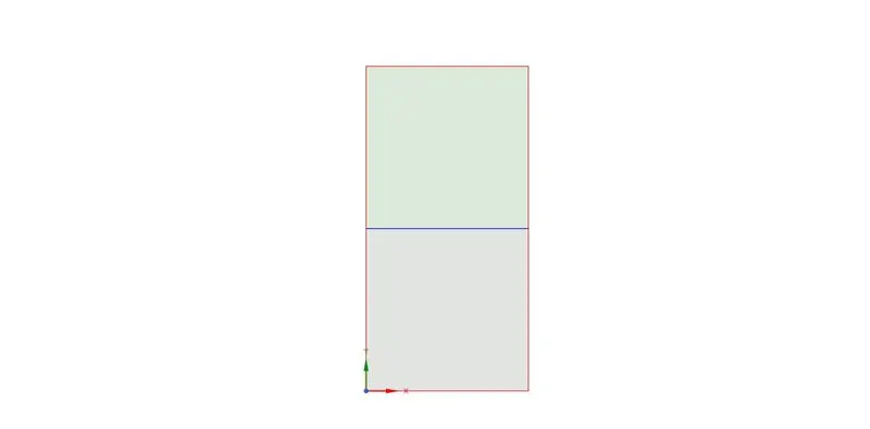
4. The top square was named as water and the bottom square was named as air.
5. Since, there are 2 different named zones, enabling the share topology option is crucial for allowing the flow of data between the 2 domains.
6. After creating this simple geometry, the model was proceeded with meshing.
7. Since the geometry is fairly simple and does not involve any complex curves, a hexahedral mesh (square mesh) was generated in the meshing tab.
8. The mesh sizes were taken as

• 0.5mm
• 0.35mm
• 0.25mm

9. All the four surfaces of the geometry were considered as wall with no inlets, outlets, and symmetry.

Setting up the case in Ansys Setup –               

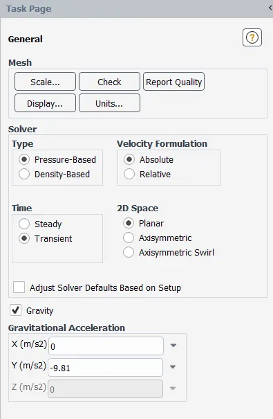
1. Since water will be dropping natural due the force of gravity, a pressure based solver was used.
2. Since we wanted to observe the results at each and every moment in time, the solution was analysed in a transient manner.
3. Furthermore, the gravity option was selected and a value of 9.81m/s^2 was put in the vertically downward y axis.
4. Since this problem does not involve measuring temperature or observing the heat flow, the energy equation was turned off
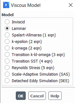
5. Since the velocity of water is very small, a laminar model was assumed for this particular case.
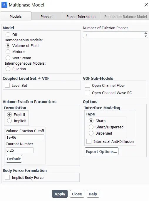
6. Also, considering that this model involves the interaction of 2 discrete phases i.e. air and water, the multiphase Volume of Fluid model was turned on.
7. Furthermore, an explicit scheme was used for solving and the default values of Courant number was considered
8. Since air and water are the 2 main fluids in this problem, water-liquid was copied from the fluent data base in the create materials section.
9. Another custom-material with properties of density = 400kg/m^3 and viscosity = 0.001 was created for 1 particular iteration.
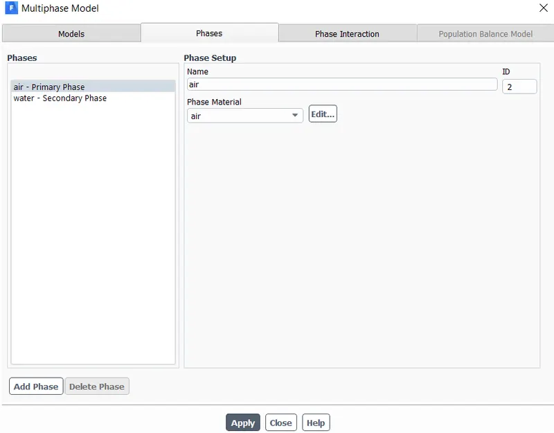
10. Next, the phases were defined in the multiphase VOF section.
11. Air was chosen as the primary phase and water was selected as the secondary phase.
12. In the final iteration, the custom-material was chosen as primary phase instead of air
13. For the boundary conditions, all boundaries were considered as walls with no inlets and outlets conditions
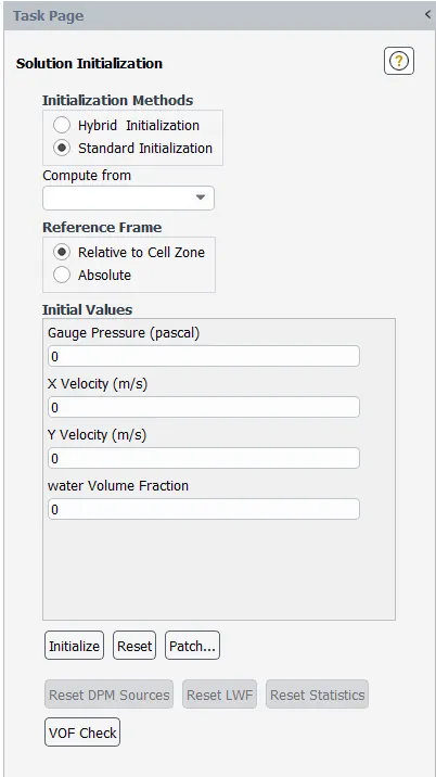
14. The solution was then initialised using standard initialisation.
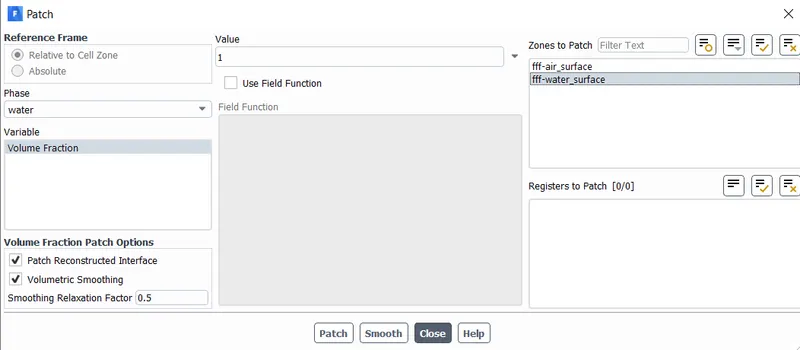
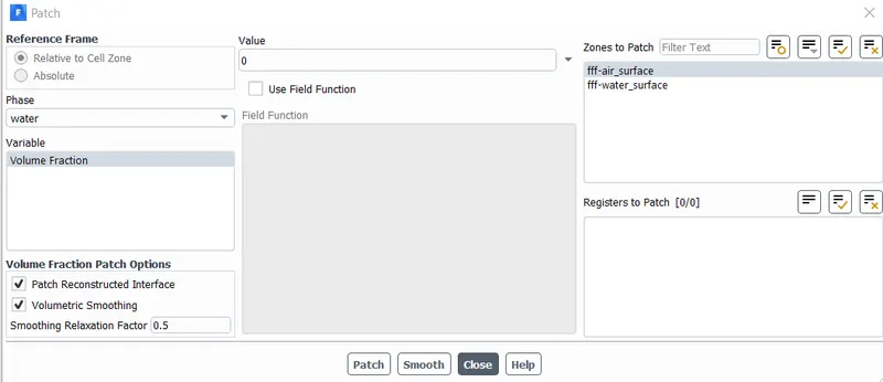
15. Another important step before running the simulations is to patch the fluid domains with respect to the volume fraction of water.
16. The PATCH option was selected and the top square area was patched with volume fraction of water = 1
17. On the other hand, the bottom area square area was patched with volume fraction of water = 0.
18. A contour plot of volume fraction of water was created on the 2D surface.
19. A solution animation of the same was created to observe the changes while the simulation runs
20. The problem was simulated using the following parameters

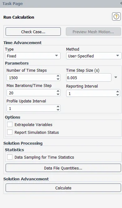
• Time steps = 1500
• Time step size = 0.005secs
• Total number of seconds = 7.5 secs
• of iterations per time step = 20

21. For more refined meshes the time step size was reduced to 0.003 or 0.002sec.

Properties of fluids –

Air - 

• Density = 1.225 kg/m^3
• Viscosity = 81 × 10^-5Pa·s

Water –

• Density = 1000 kg/m^3
• Viscosity = 001 Pa·s

Custom Fluid –

• Density = 400kg/m^3
• Viscosity = 001Pa·s

 

Results –

1. Mesh size = 0.5mm

• Primary phase – air
• Secondary phase – water
• Time step size = 0.005s
• No of time steps = 1500
  

Google drive link for animation video - https://drive.google.com/file/d/17sEqO9srnV4gJCPJcZbi2nuFSilfVkN7/view?usp=sharing

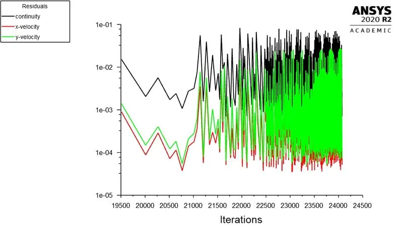
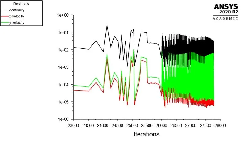
2. Mesh size = 0.25mm

• Primary phase – air
• Secondary phase – water
• Time step size = 0.002s
• No of time steps = 2000

Google drive link for animation video - https://drive.google.com/file/d/1qSdINhtQun11cUcwILFk0mdkMJcVZybu/view?usp=sharing

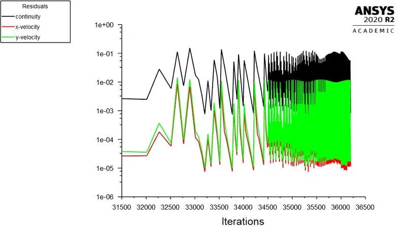
3. Mesh size = 0.35mm

• Primary phase – air
• Secondary phase – water
• Time step size = 0.003s
• No of time steps = 2000

Google drive link for animation video - https://drive.google.com/file/d/1dqsP9sfqZOP1hm0wonU9ISpSquaC8X2G/view?usp=sharing

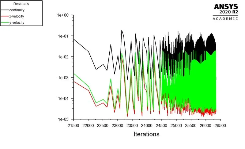
4. Mesh size = 0.25mm

• Primary phase – custom fluid – density = 400kg/m^3, viscosity = 0.001
• Secondary phase – water
• Time step size = 0.002s
• No of time steps = 2000

Google drive link for animation video - https://drive.google.com/file/d/1dn_X5htnJ4m7cjf4Cq97k95KYkBZfR0p/view?usp=sharing

Conclusions - Significance of value of Atwood number –

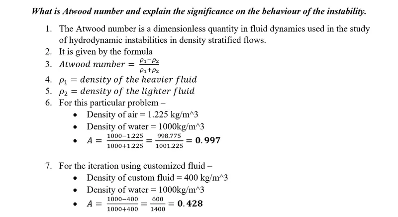
1. Since the Atwood number ranges from 0 to 1, highly different behaviours can be observed with flows at A = 0 and A = 1
2. The higher the Atwood number, the more the difference there is in the densities of the mixing fluids.
3. In this case, the mixing will occur quickly and the heavier fluid will settle down at a very faster rate.
4. The best example is air and water which we analysed in this project – A = 0.997
5. On the other hand, the lower the Atwood number, lesser the difference between density values of the mixing fluids.
6. For example, the custom fluid we generated in this project had a density of 400 which is closer to water than air is to water.
7. Hence the Atwood number came out to be very less, thus taking more time for stability since the densities were somewhat similar