Week 3 - External flow simulation over an Ahmed body.

Challenge 3 – Flow over an Ahmed Body

Aim - To analyse the flow over an Ahmed Body and study the drag coefficient based on varying y plus values and mesh refinement.

Importance of Ahmed Body –

1. An ahmed body is a research-based model used to analyse external flows over cars.
2. The ahmed body represents a standard car model from which the actual model can be optimised using the values like drag and lift coefficient.
3. The Ahmed body is a generic car body (a simplified vehicle model). The airflow around the Ahmed body captures the essential flow features around an automobile and was first defined and characterized in the experimental work of Ahmed. Although it has a very simple shape, Ahmed body allows us to capture characteristic features that are relevant to bodies in the automobile industry.
4. This model is also used to describe the turbulent flow field around a car-like geometry. Once the numerical model in validated, it is used to design new models of the car.
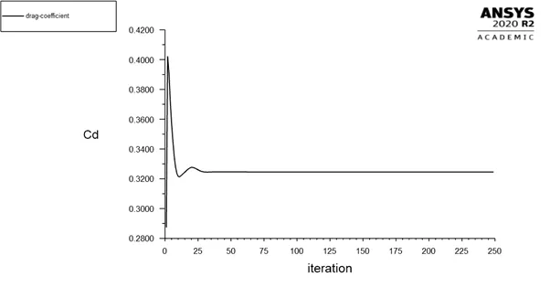
5. The drag coefficient of an ahmed body is devised to come around 0.32
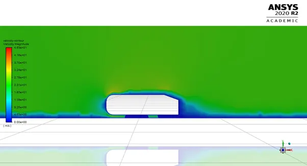
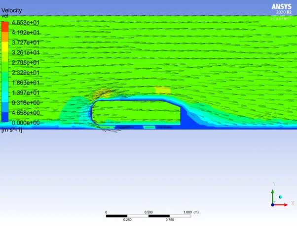
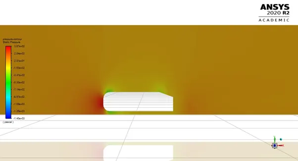
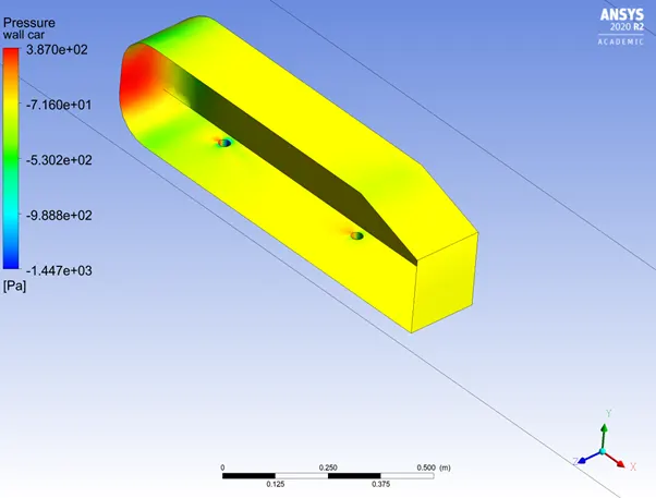
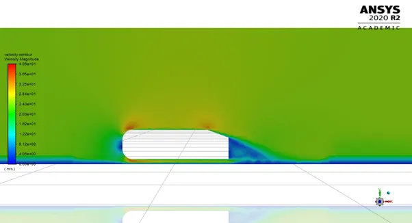
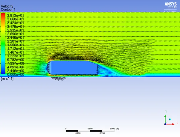
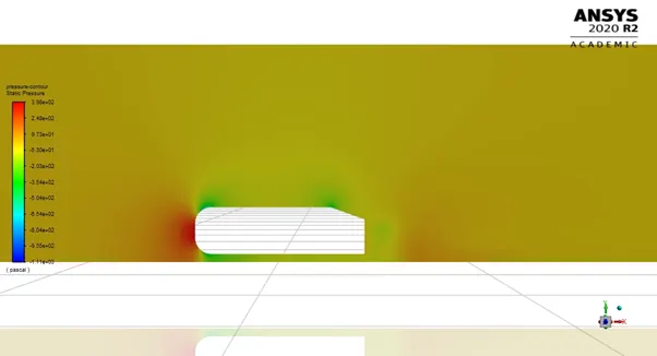
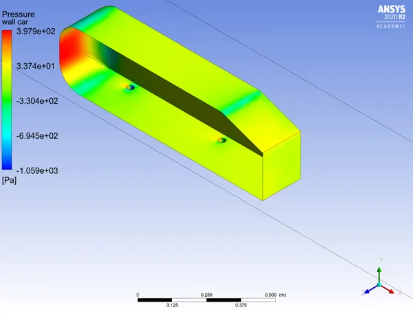
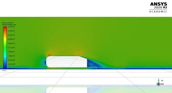
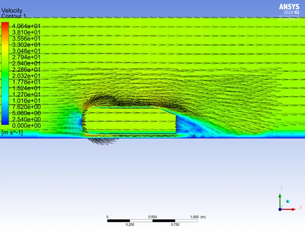
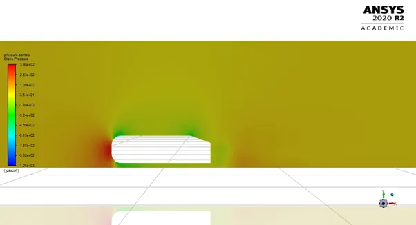
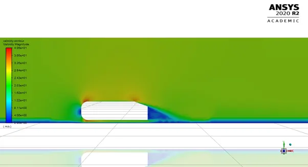
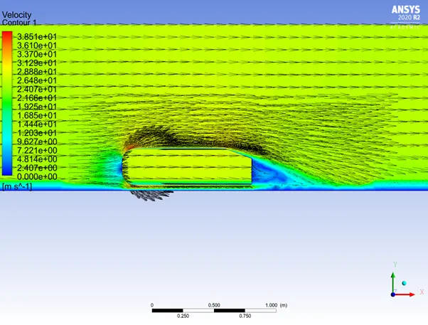
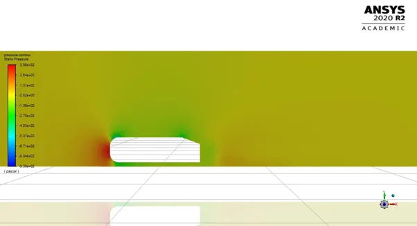
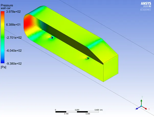
6. Other plots such as vector plots and velocity and pressure contours can be analysed to study the flow around it.

Solving and Modelling Approach –

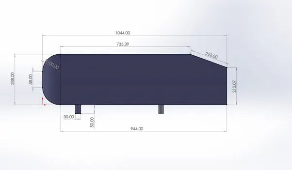
1. Firstly, the solid model of the Ahmed Body is imported into Ansys Spaceclaim.
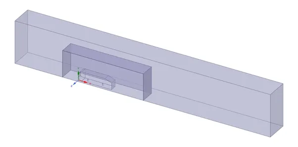
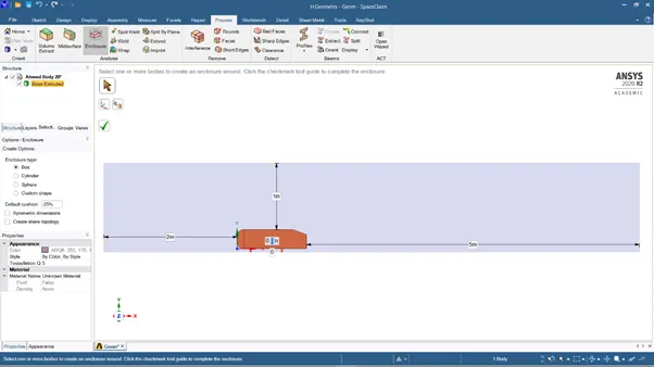
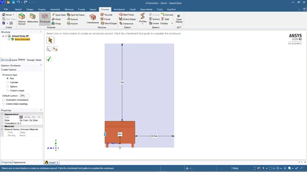
2. Since simulation is an external flow simulation, an enclosure is required to specify the fluid domain.
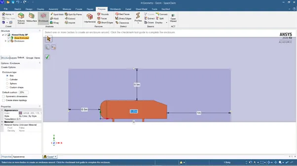
3. For the first iteration, a fluid enclosure of the dimensions as given below was created. In this iteration, a smaller enclosure (that captured minute details) was not generated since this was a baseline simulation.
4. In the subsequent simulations, an inner enclosure was created to generated a finer mesh in the portion near the Ahmed Body.
5. Using the split body command, the Ahmed Body was split into 2 symmetrical halves for the main motive of reducing mesh count and saving time required for computation.
6. Afterwards, an automatic interference check was conducted and the entire model was divided into 2 domains.
7. The Ahmed body was suppressed for physics since the fluid will flow over it.
8. Finally, share topology option was activated to ensure fluid flow and data transfer over the 2 separated fluid domains.
9. The model was then proceeded for meshing.
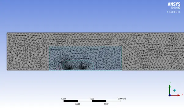
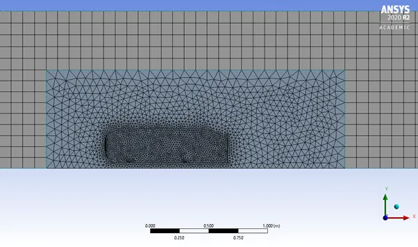
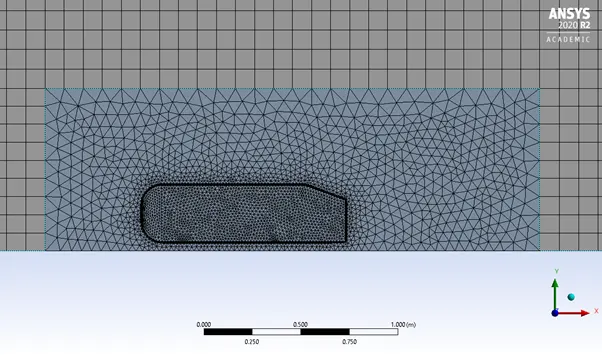
10. For the baseline mesh, a sizing of 100mm was given to the entire domain for the single enclosure.
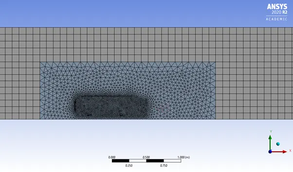
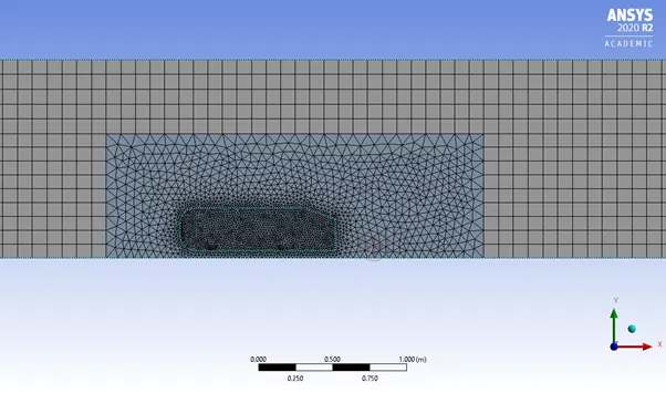
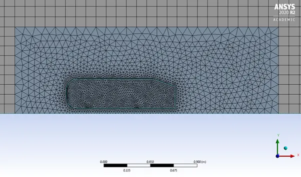
11. For the subsequent refinements, a multizone meshing method was given to the outer enclosure with a hexahedral mesh. A size of 100mm was given since this is not the main area of focus.
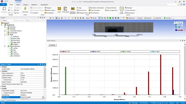
12. Furthermore, a body sizing of 40mm was given to the inner enclosure around the Ahmed body to analyse characteristics.
13. Moreover, an edge sizing was given to the cylindrical wheels to ensure that the cylinders have circular bases and do not transform into polygons.
14. Last but not the least, a local inflation layer was created around the Ahmed body surface.
15. Iterations on y+ values were carried out and the first layer thickness was calculated based on the following variables

• Free stream velocity = 25m/s
• Free stream density = 1.225 kg/m3
• Dynamic viscosity = 0.000017894 kg/m s
• Reference length = 1.044m
• y plus = varied according to iteration

16. The car body was selected using box selection and named as “wall-car” and the bottom surface was also named as a wall
17. All other faces were kept as symmetry including the velocity inlet and pressure outlet
18. The model was then further proceeded for setup.
19. Mesh settings –

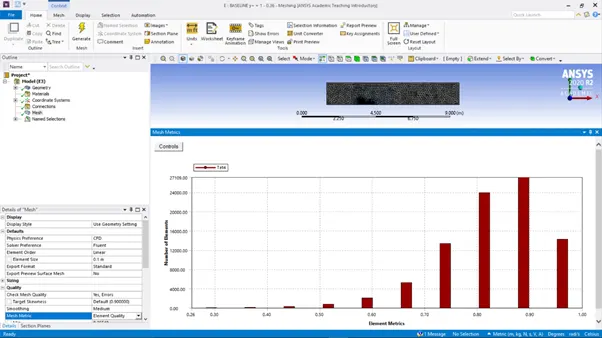
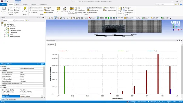
• Global mesh size – 100mm
• Method – Multizone – On outer enclosure
• Body sizing – inner enclosure – 50mm
• Face sizing – car wall – 15mm
• Edge sizing – wheel cylinders – 15 divisions
• Inflation – First layer thickness varies according to y plus values

Setting up the case in Ansys Setup –

1. Since the free stream velocity is 25m/s which around 1/13^th times of the velocity of sound, a pressure-based solver was used for the simulation.
2. The problem was analysed in a steady state manner since we are only analysing the end results
3. Since, this problem deals with wall related analysis, the k-omega SST turbulence model was chosen and the y plus value was altered between 0 – 5.
4. Accordingly, the first layer thickness was calculated using the y plus calculator and put in the inflation specifications.
5. Air which is the default material was chosen as the fluid medium in the cell zone conditions.
6. The inlet velocity was given as 25m/s in the boundary conditions sections.
7. The reference values were changed to ensure accurate values of drag and lift coefficient as well as simulation contours.
8. The frontal area was calculated using the projected surfaces tab in “Reports”, and was found to be 0.0657m^2.
9. The reference length was measured to be 1.044m and all other reference values were computed from the inlet.
10. The SIMPLE scheme was used for the solution methods.
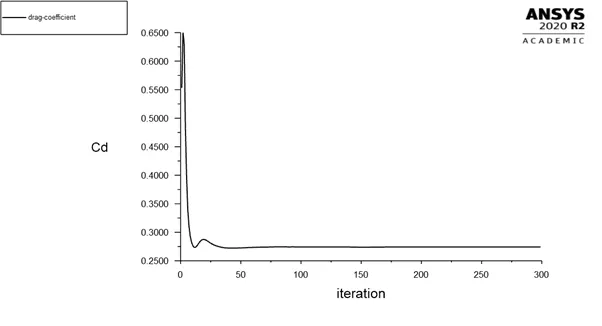
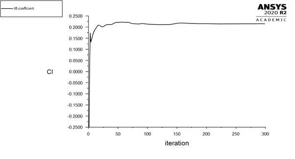
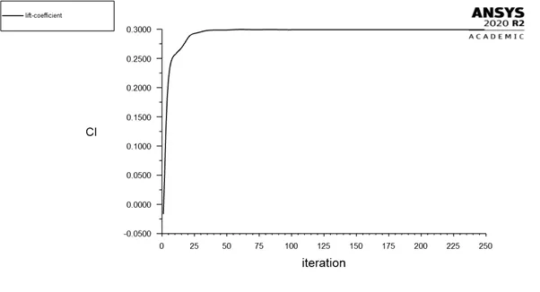
11. Furthermore, report definitions of drag and lift coefficients were generated and also printed to the console for observation.
12. A plane was created on the partition surface to analyse the velocity and pressure contours.
13. A solution animation of the velocity contour was created to observe the change in contours as the iterations proceed.
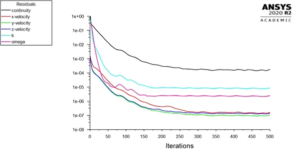
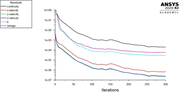
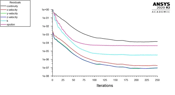
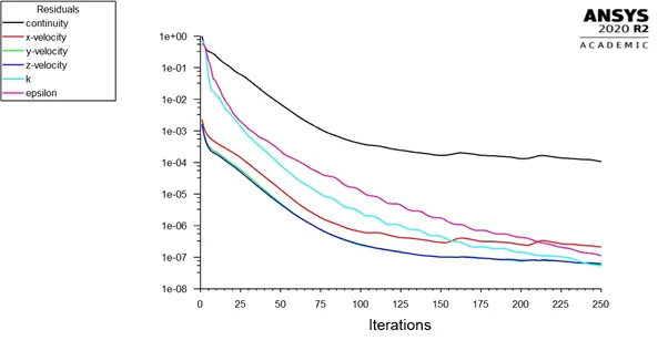
14. The solution was initialised using hybrid initialisation and run for 1000 iterations.

Results and Discussions -

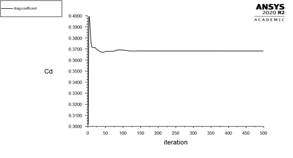
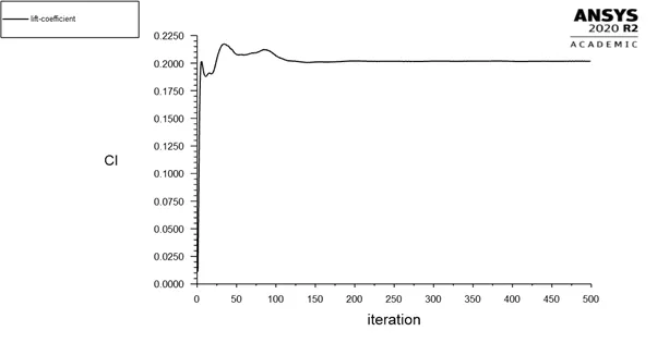
Case1 – Baseline setup – Global mesh size = 100m – NO inflation

Drag Coefficient – 0.36

Case2 – Y+ = 1 --- K-omega SST Model

First layer thickness = 0.00001432966469389308m

Drag Coefficient – 0.25

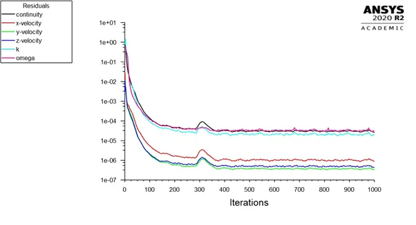
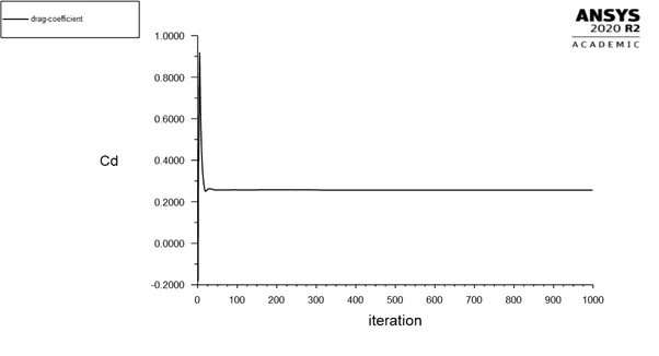
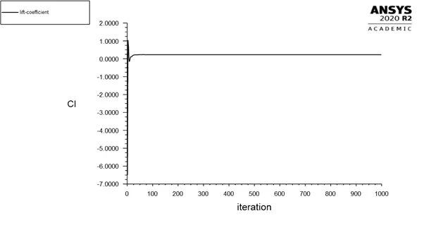
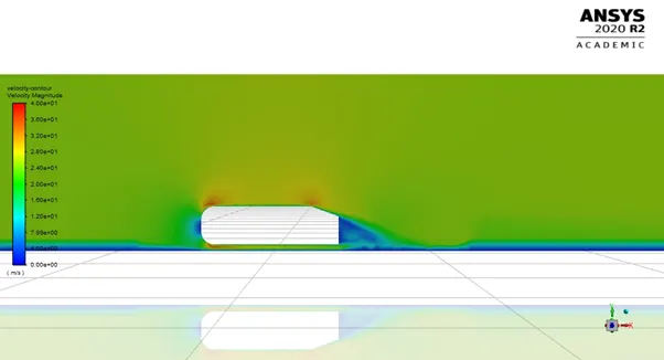
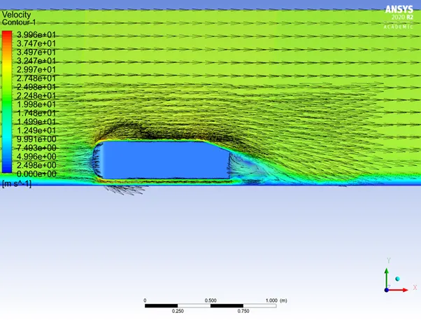
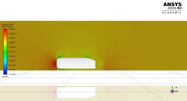
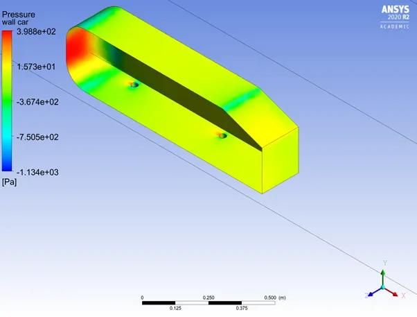
Case3 – Y+ = 3 --- K-omega SST Model

First layer thickness = 0.00004298899408167923m

Drag Coefficient – 0.27

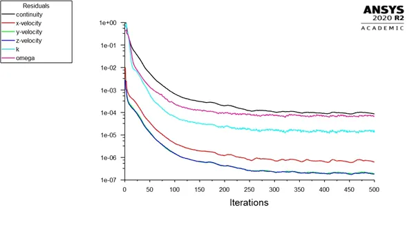
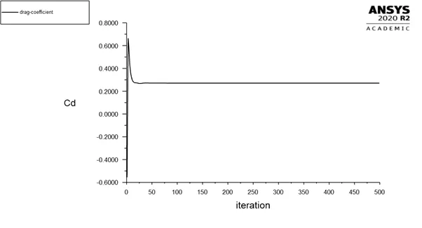
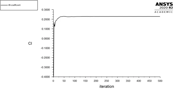
Case4 – Y+ = 5 --- K-omega SST Model

First layer thickness = 0.0000716483234694654m

Drag Coefficient – 0.28

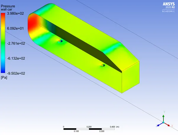
Case5 – Y+ = 30 --- K-epsilon Standard wall functions

First layer thickness = 0.00042988994081679234m

Drag Coefficient – 0.31

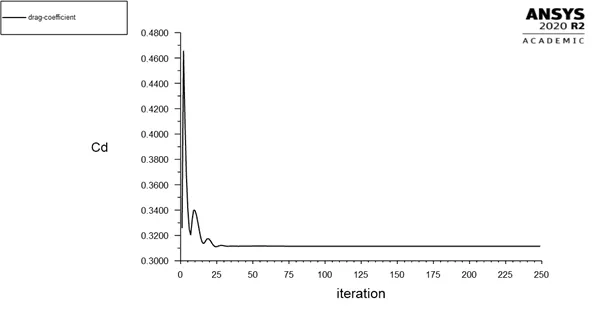
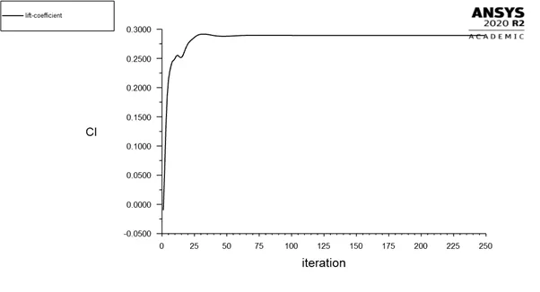
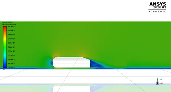
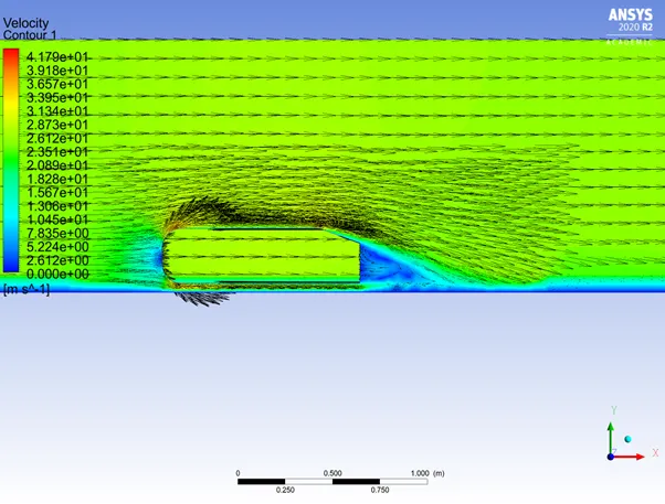
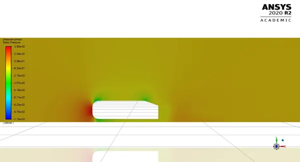
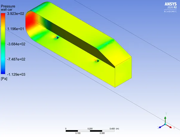
Case6 – Y+ = 100 --- K-epsilon enhanced wall functions

First layer thickness = 0.001432966469389308m

Drag Coefficient – 0.32

Conclusions and Inferences –

1. The k epsilon model proved to get accurate results of drag coefficient of about 0.32.
2. Since this particular model is not better than SST k-omega model for wall related problems, a y plus value of greater than 30 was kept with 2 iterations at 30 and 100.
3. On the other hand, the K-omega SST model gave values of drag coefficient close to 0.25

Reasons for pressure becoming negative –

1. As the air flows over an ahmed body, the velocity increases rapidly. SO, thus the pressure reduces to values below 0 to maintain the flow pattern.

Reasons for flow separation –

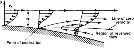
Flow separation or boundary layer separation is the detachment of a boundary layer from a surface into the wake region.

Separation occurs in flow that is slowing down, with pressure increasing, after passing the thickest part of a streamline body or passing through a widening passage

References –

1. https://www.researchgate.net/publication/266883948_Flow_and_Turbulence_Structures_in_the_Wake_of_a_Simplified_Car_Model_Ahmed_Model
2. https://www.researchgate.net/publication/330383775_Experiments_and_numerical_simulations_on_the_aerodynamics_of_the_Ahmed_body