Week 6 - CHT Analysis on a Graphics card

Objective:

In order to simulate a forced convection flow on a graphics card and investigate the conjugate heat transfer that occurs during the simulation, to carry out mesh independent research, and to evaluate and evaluate the results of these investigations. We are going to run simulations at three different speeds: one metre per second, three metres per second, and five metres per second. For the simulation at three metres per second, we are going to use a finer mesh.

Conjugate Heat Transfer (CHT) analysis :

Using an analysis technique called "conjugate heat transfer," one may model the flow of heat from one domain (solid or fluid) to another (through conduction inside the solid and convection within the fluid) and back again. By simultaneously solving all of the pertinent processes involved in solid and flow field heat transfer, conjugate heat transfer analysis is able to properly forecast how heat will be transferred. The combination of heat transfer in solids and heat transfer in fluids is what's meant to be understood by the term "conjugate heat transfer." While convection typically takes the lead in fluids, conduction tends to be the dominant form of heat transfer in solids. It is possible to witness conjugate heat transfer in a variety of contexts, such as in the case of conduction through solids, free and forced convection in gases and fluids, and thermal radiation.

The three primary means by which heat is transferred are as follows:

The process of heat transfer that takes place when there is a temperature difference across a stationary medium is referred to as conduction. The process of heat transmission that occurs when there is a disparity in the temperatures of a surface and a fluid that is moving is referred to as convection.
The emission of energy in the form of electromagnetic waves is what we refer to as radiation (also known as thermal radiation). There is a positive net heat transfer by radiation between two surfaces that are different temperatures when there is no intervening medium in the path between them.

Conduction :

The transfer of heat energy through a solid or fluid occurs by a process known as conduction. This process is driven by the translational, rotational, and vibrational motion of atoms and molecules. Collisions between molecules are what transmit energy from highly energetic molecules to those with less energy. The higher the temperature, the more atomic and molecular mobility there will be. Conduction can take place in any medium, be it solid or liquid.In accordance with the Second Law of Thermodynamics, heat must invariably move from locations of greater temperature to those of lower temperature. When there is an issue with conduction, it frequently involves fluid flows at the boundary of the solid. These fluid flows act as a mechanism for either heating or cooling the solid. Because of the difference in temperature, energy can be transferred from more energetic particles of a substance to less energetic particles of that substance via interactions between the particles on molecular levels. This process is known as conduction. There is a correlation between the energy of random translational, internal rotational, and vibrational motions of gas molecules and the temperature at any given place in space.

Energy is transferred from highly energetic molecules to less energetic molecules as a result of collisions between molecules. When there is a temperature gradient present, the transfer of energy always occurs in the direction of decreasing temperature. This is because larger molecular energies are associated with higher temperatures, and the transfer of energy always occurs in the direction of decreasing temperature. Because the molecules in liquids are closer together and their interactions with one another are greater and more frequent than in gases, the process of conduction is the same for liquids as it is for gases. When it comes to solids, conduction is linked to atomic activity that manifests itself as lattice vibrations. In the case of an electrical conductor, another factor that contributes to the movement of free electrons and the consequent transfer of energy is translational motion. The process of heat transfer can be quantified using the proper rate equations, which are then used to quantify the amount of energy that is being transported per unit of time. Fourier's law can be thought of as the rate equation for the process of heat conduction. This is represented mathematically for a one-dimensional plane wall as

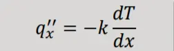
In this context,

the rate of heat transfer per unit area in the x-direction is denoted by "q x" (W/m2)
k is the thermal conductivity, measured in W/mK, and it is a property of the material that makes up the wall.
The fact that the heat transfer is going in the opposite direction of the temperature gradient is denoted by the negative sign.

The process of convection:

Convection is the process of heat transfer that occurs when the bulk motion of a fluid is combined with the random molecule mobility of the fluid (diffusion). Conduction at the walls allows heat to be transmitted either into or out of the fluid. The fluid distributes the system's thermal energy to the various other components. Advection is the term used to describe heat transfer that occurs only as a result of the bulk motion of the fluid and does not involve diffusion.

There are three categories that convection heat transfer can be placed in:

Forced convection: Flow is produced by an external agent, such as a fan, a pump, or the natural winds in the environment.
The flow is produced by buoyant forces, which are caused by differences in density that are attributable to the temperature variations in the fluid. This type of convection is known as free (or natural) convection.
Convection can be either forced or natural, or both, if there are driving forces from the outside and buoyant forces within the system.
The concept that the rate of heat transmission is directly proportional to the temperature gap that exists between a fluid and a heated or cooled body is the foundation of the convection method of heat transfer.
Newton's Law of Cooling is the name given to this theory. The heat transfer coefficient, which is typically indicated by the symbol h, is the variable that determines the rate at which heat is transferred.

Here, 𝑞′′ = Convective heat flux
𝑇𝑠= Temperature of the solid surface
𝑇∞= Temperature of the fluid

The calculation of the heat transfer coefficient for a specific flow field is one of the most important aspects of the convection process.
The heat transfer coefficient is determined by the conditions that are present in the boundary layer. It is also influenced by the geometry of the surface, the characteristics of the fluid flow, and a number of other thermodynamic and transit characteristics of the fluid.

Transfer of Heat Via Radiation:

Producing heat via emitting radiation The emission of energy in the form of electromagnetic waves is what constitutes heat transfer. When heated above absolute zero, every particle of matter releases heat in the form of thermal radiation.
This emission occurs because of shifts in the electron configurations of the atoms or molecules, and electromagnetic waves are responsible for the transmission of the energy (or photons). The intensity of radiation is influenced both by the temperature of the body and the features of the surface. Radiation, on the other hand, does not rely on the presence of a material medium and can take place even in a vacuum. Conduction and convection are two more forms of heat transfer. At high temperatures, one of the most important ways heat is transferred is by radiation.
In addition to this, it is the only method of heat transfer that is possible in space, which is how solar energy is brought to Earth. The majority of applications mix heat transfer in solids and heat transfer in fluids to get their desired results. This occurs because to the fact that fluids can flow around solids or between solid walls, and also due to the fact that solids are typically submerged in a fluid. The analysis of temperature fields and heat transfer is made possible by providing a detailed description of the modes of heat transfer, the properties of the materials, the flow regimes, and the geometrical configurations. A description of this kind can also serve as the basis for a numerical simulation, which is a tool that can be used to forecast the effects of conjugate heat transfer or to test various configurations in order, for instance, to optimise the thermal performances of a particular application.

Introduction :

We are going to perform a steady-state conjugate heat transfer analysis on a model of a graphics card by using aluminium for all of the materials that are not the processor. We are going to do this because aluminium is used to create an efficient fin formation medium for transferring heat in a variety of industrial and heat transfer applications. In this case, we are going to use it to model a graphics card. Aluminum is selected as the material of choice due to the inherent light weight, increased conductivity, and easy malleability of the material. Because it is naturally resistant to corrosion, it is also a better choice for applications in which it will be exposed to the environment, liquids, or chemicals. This is because corrosion can be caused by a number of different factors. Aluminum fin stock is the material of choice for radiators, evaporators, coolers, heaters, and condensers in a variety of industries, including aerospace, automotive, and heating, ventilation, and air conditioning. This is due to the properties discussed above.
And for processors, we use silicon, which is used for electronic devices because silicon is a material that possesses very special properties and is therefore used for these devices. The fact that it functions as a semiconductor is among its most valuable characteristics. This means that under certain conditions it acts as a conductor of electricity, whereas under other conditions it acts as an insulator. Doping is a process that can be used to change the electrical properties of silicon. Because of these properties, it is an excellent material for the production of transistors, which are devices that amplify electrical signals. Silicon is an excellent material for use in electronic devices for a number of reasons, not the least of which is due to its properties. Silicon is another element that can be found in high quantities on Earth. It is even the element that makes up the most of the crust of the Earth. Because it is so abundant, silicon is relatively inexpensive, making it a desirable material. It should come as no surprise that silicon has become the primary component of memory chips, computer processors, transistors, and virtually every other type of electronic device.
The central processing unit (CPU) converts the energy of any electricity that flows through it or that is blocked within it into heat. In a high-performance workstation, it is possible for the processor to overheat due to heavy use; however, in a regular computer, a processor that overheats is almost always an indication that the system is not functioning properly. Therefore, it is essential for the cooling of the processor.
Because the fins are attached to the processor, the heat from the processor is conducted to the fins, and then the heat is removed from the processor by using air as a coolant and forced convection to remove heat from both the processor and the fins to cool the processor.

Methodologies for Solving and Modeling:

In accordance with what was covered in Aim, we will solve for four different cases.

We will be creating the geometry and performing unstructured tetra CFD mesh with boundary definitions using the ANSYS Fluent solver. After that, we will setup the physics of fluid flow and run the iterations to get solutions. Finally, we will use post processing to interpret the data in the form of plots, contours, vectors, streamlines, and other such things.

We are going to investigate grid independence for CHT analysis of the exhaust port using RANS using a velocity of 3 metres per second. When we talk about the grid independence study, we mean that we are going to look at the following four cases.

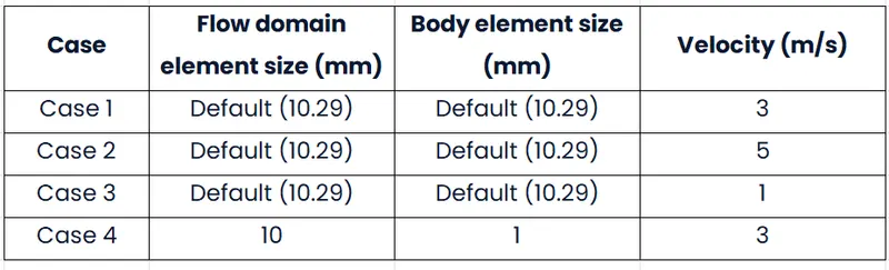
Because we are working with a student edition of ASNYS, we will be restricted in the number of variables we may experiment with. Then, to ensure the simulation is accurate, we compile a database of the case study's findings and compare them to those found in publicly available literature or published book data.

Preprocessing and Solver setting:

Let's launch the ANSYS workstation right now. You can either double click on the Fluent button or use the drag-and-drop feature in the schematic window to create fluid flow. Steps like

GEOMETRY > MESH > SETUP > SOLUTION > RESULTS

make up the streamlined procedure. Before moving on to the next phase, you will need to finish each step in its entirety.

Case 1 will be discussed in depth in the grid independence study.

GEOMETRY >

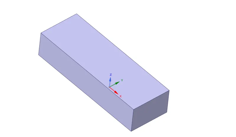
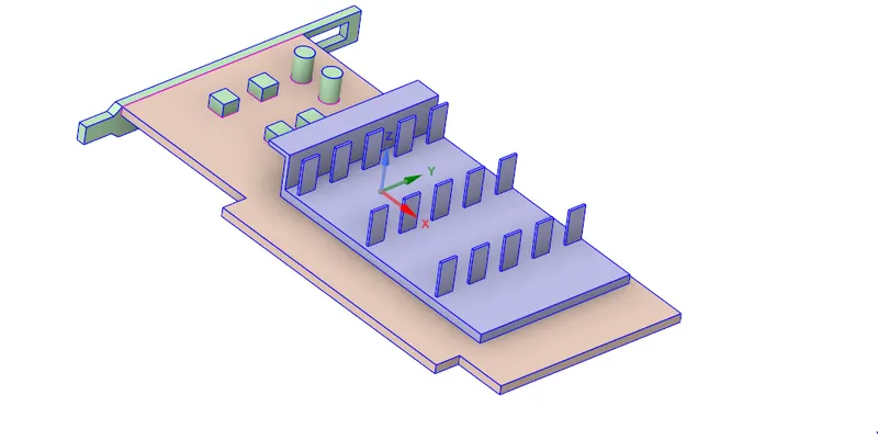
To create a new SpaceClaim Geometry in the Fluent, right-click on the Geometry icon, and then select the option. After opening the space claim application, go to the 'File' menu and then 'Open' to access the Graphics card model. It is plain to see that the model already incorporates a housing of some kind. We need to run the SHARE TOPOLOGY command in order to ensure that the fluid volume and the solid volume will interact with one another's nodes. Following the completion of the share topology procedure, we can promptly save the file.

We are all set to go at this point. As soon as the geometry is ready, we are able to close the space claim and verify that the fluid flow geometry has been updated, as indicated by a green tick.

MESH >

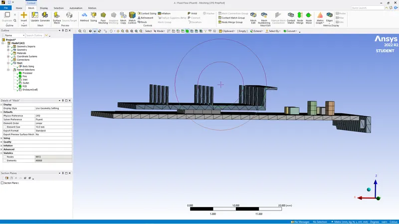
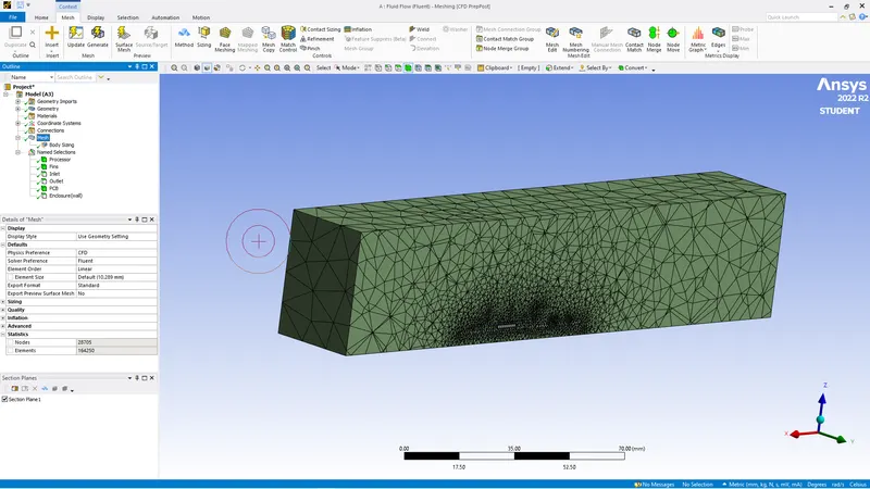
The Mesh window can be opened by selecting edit from the context menu after right-clicking on the Mesh. Because the Mesh window is already loaded with the geometry that we have been working on, clicking the GENERATE MESH button ought to cause an automatic generation of a mesh.

The default mesh size for this location is 10.29 millimetres. The elements are found in a mixed state in nature, which means that we obtain tetra elements for fluid volumes and quad elements for prismatic structures; the total number of elements is approximately 80,000.

Whenever the user makes a modification, they should either click the update icon to reflect the modifications in the mesh's specifications or a lightning bolt symbol will appear to remind them to do so.

We are going to give the surfaces that lead into and out of the room names like Inlet, Outlet, and Wall. To do this, we are going to select the outer faces of the model, then press the "N" button. We will choose the bodies, and we are going to give them the names PCB, Fins, and Processor in that order. When this is finished, we should notice a green tick somewhere close to Mesh. It is possible for us to shut the mesh window.

SETUP >

The Fluent launcher is opened by right clicking the Setup. Select 3D, Double Precision, and the number of cores based on the user's system configuration in the Fluent launcher, then click Start.

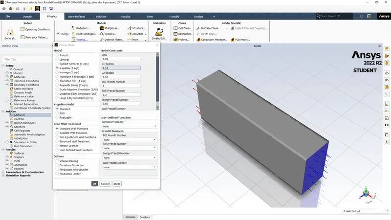
As soon as the programme is opened, choices must be made in order to define the definitions for the simulation. We will choose Type: Pressure based, Velocity Formulation: Absolute, and Time: Steady. We can enable viscous and choose k-omega > SST under the Physics tab. Activate Energy.

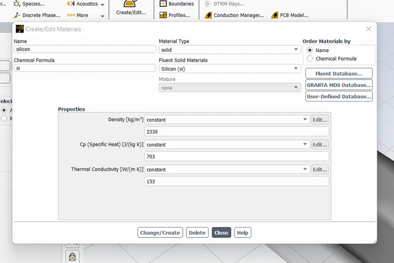
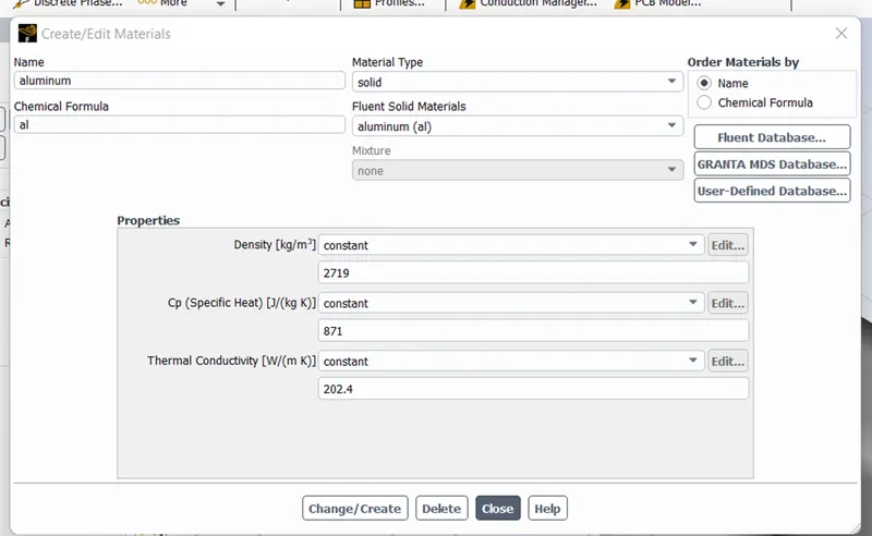
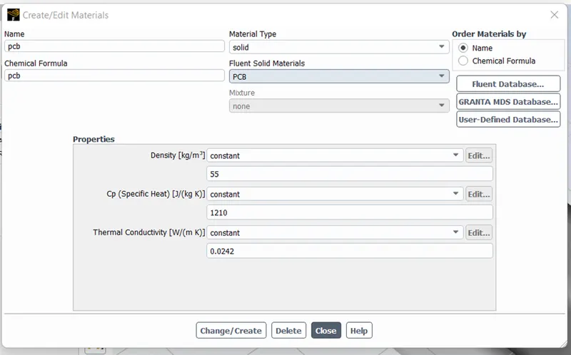
We'll choose air as our default material under the materials heading with fluid as the material type. We will take into account the solid volume as well, using aluminum as the default solid material since we are dealing with the CHT analysis. By copying the aluminum and changing the properties like density, specific heat, and thermal conductivity from standard data books for materials as follows, we can add two more materials for the processor and the PCB.

When the cell zone conditions are met, choose the solid volume, verify that the material selection is solid, and then choose the fluid material for the fluid volume. When using the processor, after choosing the material, make sure source term is enabled and input 31250000 W.

Q = 2 W, Qg = Q/V

V = 8*8*1 e-9

Qg = 2/64 = 31250000 W/m^3

& boundary conditions, as follows

Inlet : velocity magnitude = 5 m/s

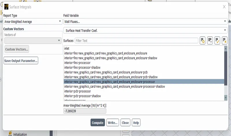
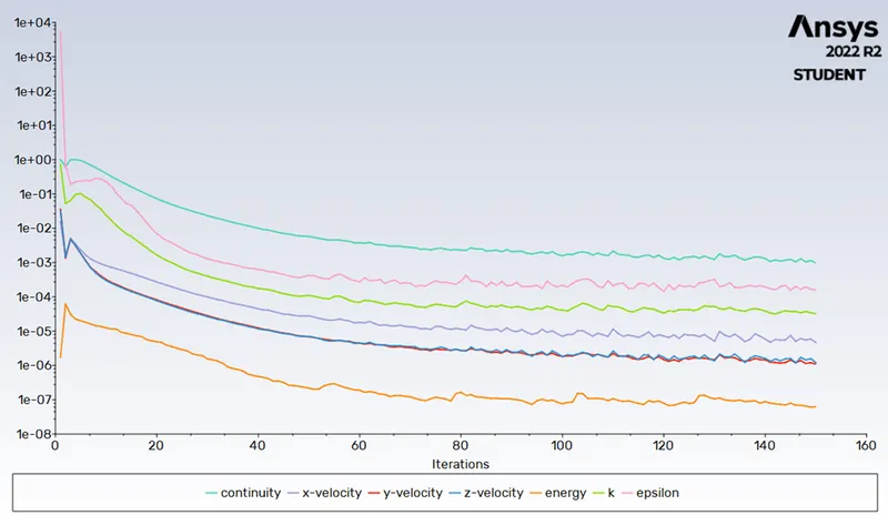
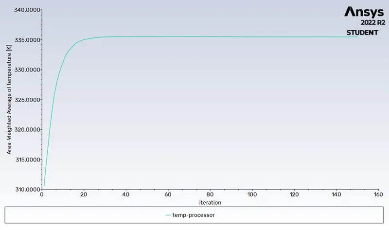
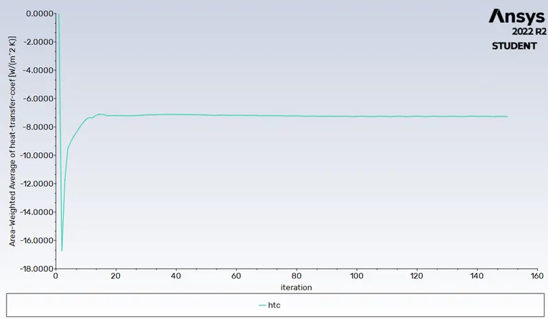
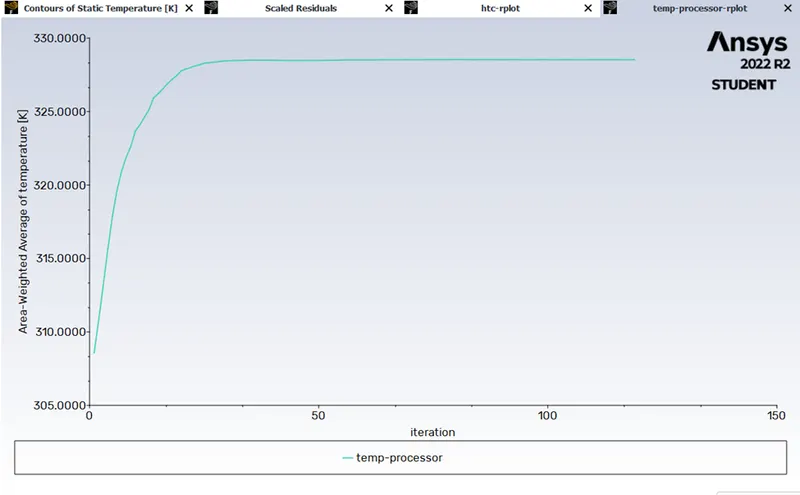
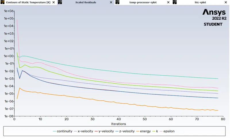
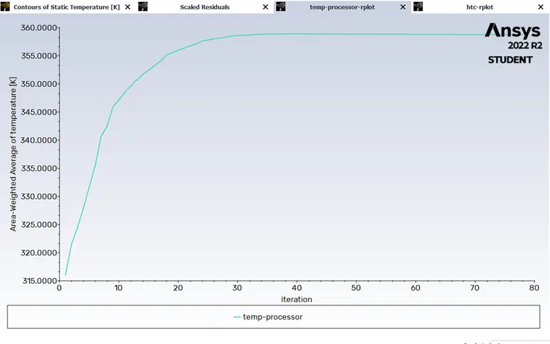
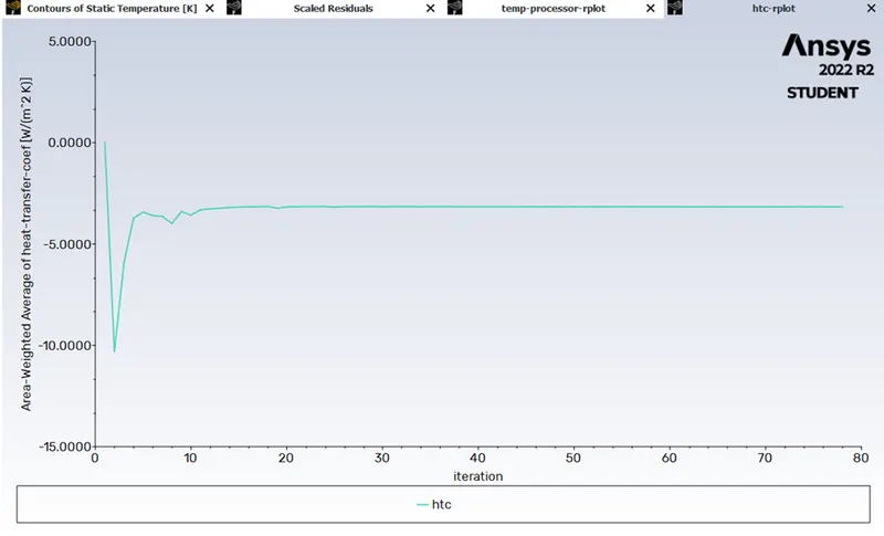
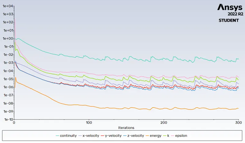
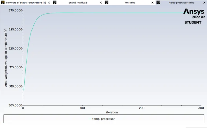
Click on the Solution > Reports > Definitions > New > Surface Report > Area weighted average > Wall fluxes > Surface heat transfer coefficient in the processor to generate surface reports. For more information regarding the heat transfer coefficient, see the Surface heat transfer coefficient. In addition, produce a separate report that focuses on the temperature of the processor. Now is the appropriate time to initiate the simulation. To begin the simulation for the physics that have been set up above, we must first initialise the entire flow field by clicking on the t=0 initialise icon. This will allow us to start the simulation. In the section labelled Run Calculation, we are able to enter the desired number of iterations (150 in this case), and clicking on the Calculate button will hopefully begin the iterations. After a certain number of iterations, we will have scaled residuals, a plot of the average temperature, and a plot of the surface heat transfer.

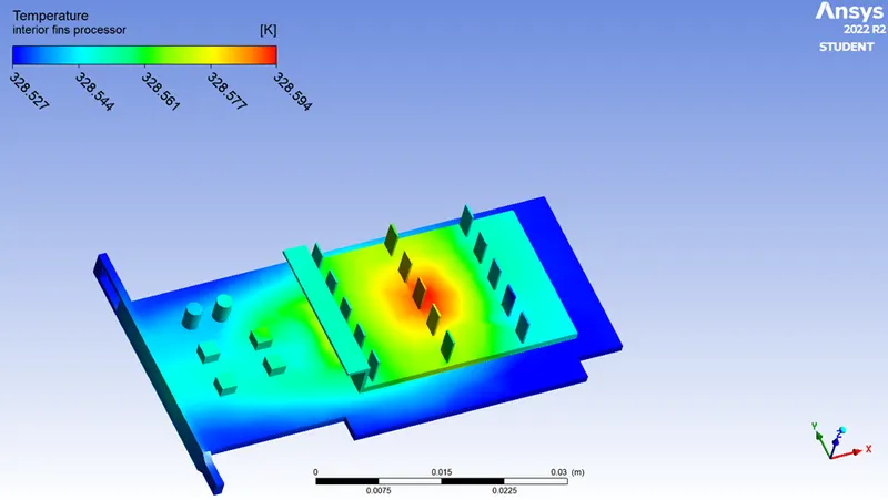
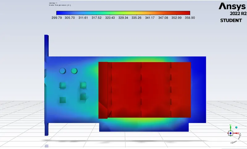
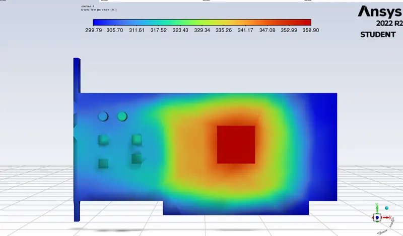
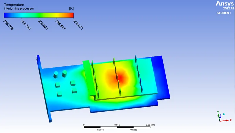
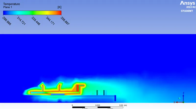
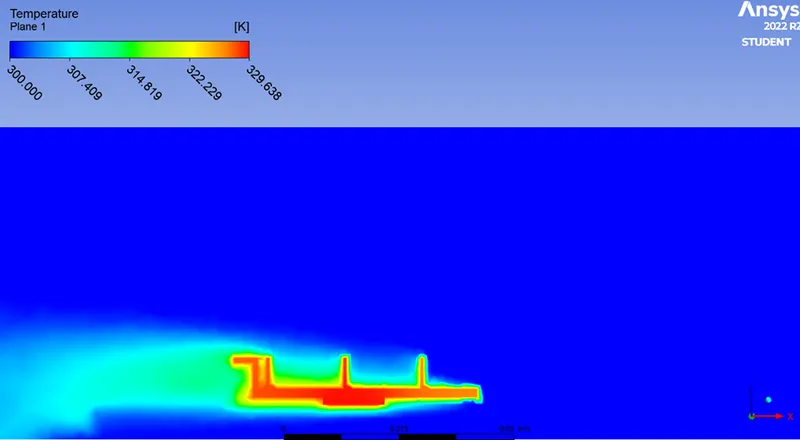
We also need the temperature contour, and in order to get it, we need to colour the bodies to make a new contour in the Results > Graphics > Contours > New temperature menu option. Simply double clicking on the scale will bring up the editing options.

If you are viewing the simulation reports in the Outline view, clicking on the Report Outline > Generate button should produce an Ansys Fluent Simulation Report. This report is automatically generated and contains all of the information regarding the simulation. Additionally, a PDF version of this can be generated. Since we are finished with the setup, you may now close it.

SOLUTION >

Because some of the solution is already calculated when the setup is being created, we can observe the green ticks in both the setup and the solution as well.

RESULTS >

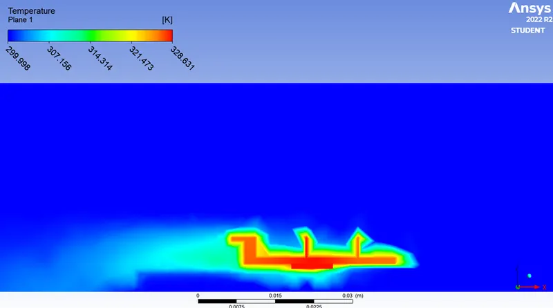
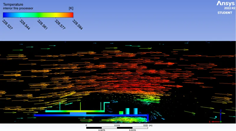
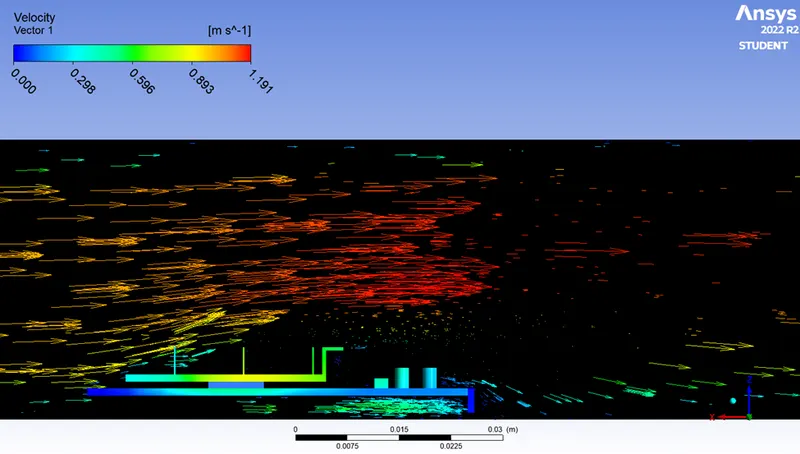
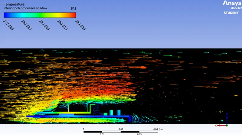
If you click the Results with the right mouse button, the Post processor should open. The default view is a wireframe model, and within XZ, we can create a plane to view contours and vectors in the model. A velocity vector is created by selecting both the Vector and the plane at the same time.

In a manner analogous to that of setup and solution, all plots and contours can be generated in this section. Furthermore, we have the ability to generate an animation of the velocity contour by first clicking on AUTOSAVE during the solution, then clicking on ANIMATE, and finally selecting the make movie option before saving the file in the location of our choosing.

In Cases 2 and 3, we will proceed in the same manner, with the exception that we will alter the velocity in the boundary conditions. We need only make a DUPLICATE of the case 1 fluent file in order to make any necessary edits.

For Case 4, we need to refine the mesh for bodies to 1 millimetre while keeping the fluid domain mesh size at 10 millimetres; other than that, all of the steps are the same as they were for Case 1.

OUTCOMES:

Following the execution of the same simulation procedures across all of the cases derived from aim, we now have a number of data that can be compared and investigated. We are going to organise all of the contours, plots, and vectors so that we can examine them side by side and reach a decision. Only the results of all of the cases are shown here; the inferences and interpretations based on those results will be briefly discussed before the conclusion.

Case 1

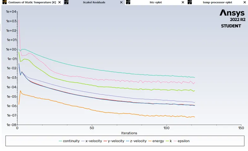
Residual Plot

Temp Plot

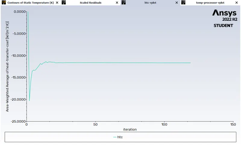
htc plot

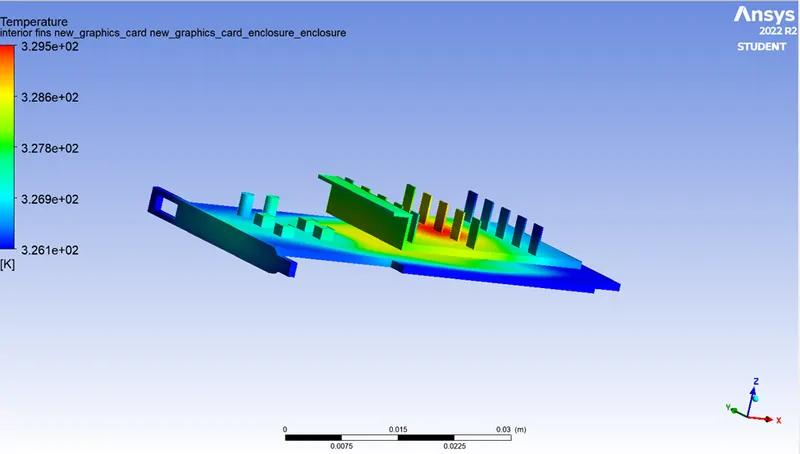
Contour Plots of different parts

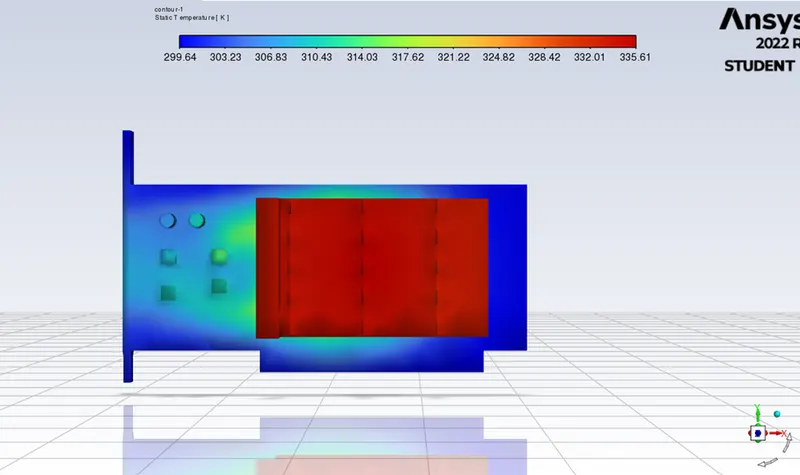
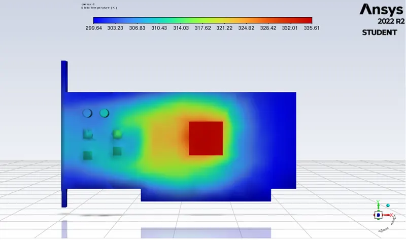
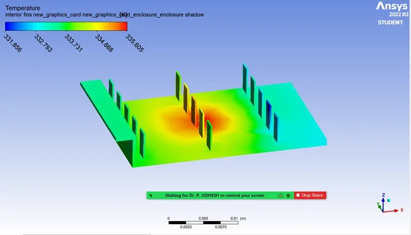
Temp Plots

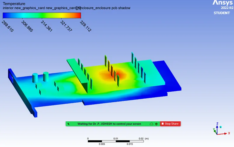
Temp Plot with PCB

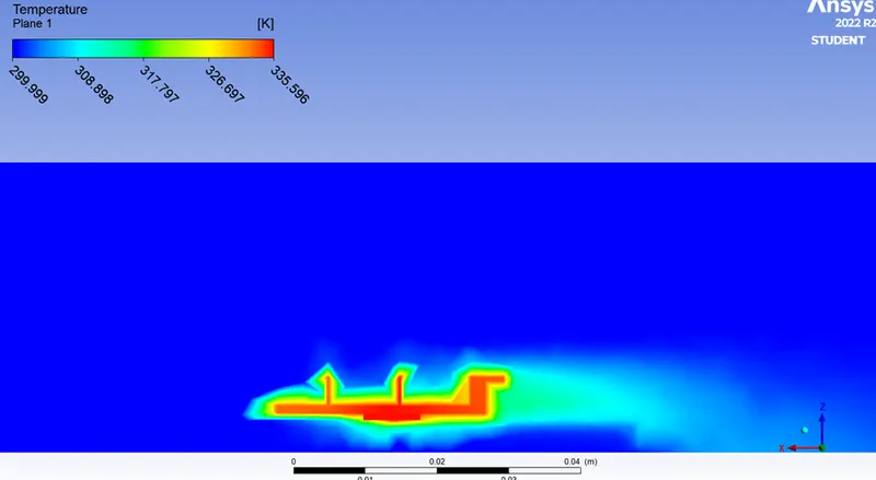
Temperature contour

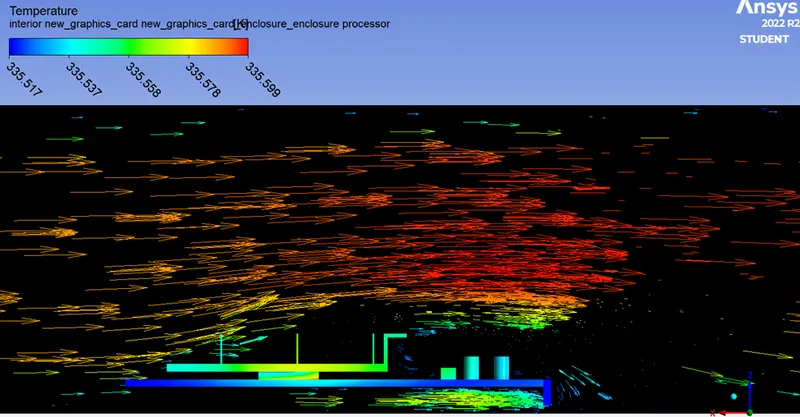
Velocity vector

Case 2

Case 3

Case 4

CONCLUSION:

Let's create a table using the findings from all four scenarios to determine the surface heat transfer coefficient and the maximum temperature of the processor, along with the appropriate grid sizes and speeds.

Grid Size	Case 1	Case 2	Case 3	Case 4
Flow domain mesh (mm)	10.29	10.29	10.29	10
Body mesh (mm)	10.29	10.29	10.29	1
No.of elements	8268	8268	8268	190486
Surface heat transfer coefficient (W/m^2.K)	-7.269	-11.67	-3.166	-10.17
Maximum temperature of processor (K)	335.48	328.52	358.76	329.48

It is clear from this that the heat transfer coefficient has a direct relationship with the velocity at which the fluid is introduced into the system. Additionally, an inversely proportional relationship exists between the maximum temperature of the processor and the inlet velocity. In terms of the heat transfer coefficient, there is not a significant difference between coarse and fine mesh; however, the maximum temperature that can be reached is greater in coarser mesh. When compared to 1 and 3 metres per second, the velocity of 5 metres per second is optimal for cooling.

INFERENCES:

As a result of the grid independency study, we have learned that the results obtained by using a finer or coarser mesh are almost identical. When using a finer mesh, however, as opposed to the coarse mesh used in cases 2 and 4, the back flow vortices become readily apparent during the post-processing stage.

Since the finer size mesh elements don't have a significant impact on the surface heat transfer coefficient, using a finer mesh results in the processor reaching a lower maximum temperature.

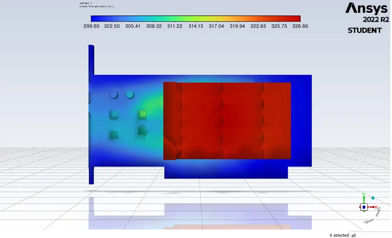
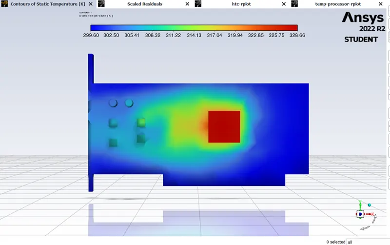
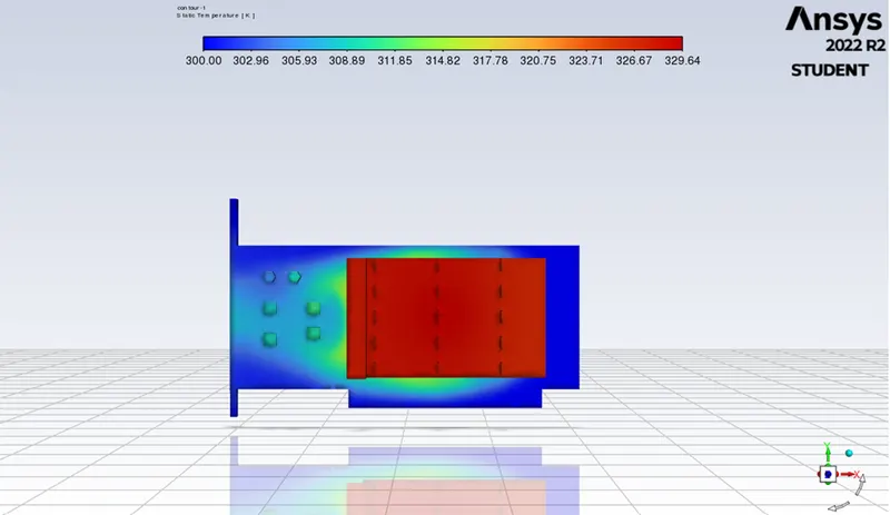
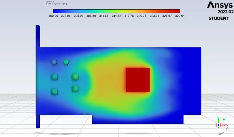
We can see from the temperature contours that the average temperature of the PCB is much lower when compared to the temperature of the fins. This is due to the material properties, such as low thermal conductivity, that the PCB possesses. This heat-affected region of the PCB can be seen in the temperature contour without fins, which shows that at low velocities, the heat-affected region has a large surface area. Because of this, there is a risk that the PCB will overheat and fail. Therefore, in order to keep the temperature of the processor stable, we need an adequate inlet velocity, which in this instance should be at least 5 metres per second.

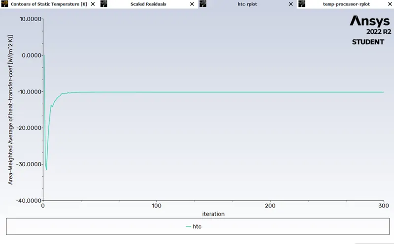
Because the source has reached its peak temperature, the plot of the surface heat transfer coefficient has increased before it has reached a steady state. This is the cause of the phenomenon. As the simulation begins with an initialization value of zero, the processor quickly reaches its maximum temperature. Simultaneously, the air velocity begins to pick up, and the rate of heat transfer eventually stabilises at a value that is constant across all four scenarios. The maximum point on the plot is determined by how fast the air is entering the system.