Week 6 - CHT Analysis on a Graphics card
CHALLENGE - 6: CHT Analysis on a Graphics Card
AIM:
To perform the simulation of Conjugate heat transfer analysis on given graphics card geometry by using ANSYS FLUENT.
OBJECTIVE:
- To study the importance of Conjugate heat transfer analysis.
- To perform the simulation of Conjugate heat transfer analysis on given graphics card geometry by using ANSYS FLUENT.
- To calculate the maximum temperature and heat transfer coefficient attained by the processor.
- To plot different temperature contours of baseline and fine mesh simulations by varying the inlet velocities..
THEORY:
Conjugate Heat Transfer Analysis -
Conjugate heat transfer analysis (CHT) describes the heat transfer due to the interaction of a solid body and fluid flowing over or inside it. Conjugate heat transfer plays a vital role in the modern world ranging from automotive industry, aerospace, cryogenic applications, food processing, cooling of electronic devices, Heat exchanger design etc. CHT analysis provide the temperature distribution, heat transfer contours, heat transfer coefficient, heat flux values at the interface thus one can easily conclude the behaviour of a system.
Materials which are considered for the simulation are:
Processor - Silicone
Fins - Copper
Base - Acrylonitrile butadiene styrene (ABS plastic)
Constant heat generation is considered on processor
The value of heat generation is
`underset(g)dotq=Q/V`
Where Q = 1W
V =Volume of processor= 8mm*8mm*1mm = 64mm^3 = 6.4*10^-8 m^3
=> Heat generation = 1/6.4*10^-8 = 15625000 W/m^3.
PROCEDURE:
1. Open ANSYS Workbench 2022R2 select Fluid Flow (Fluent) from Toolbox.
2. Rename the file and left click Geometry and select New Spaceclaim Geometry.
3. Open the geometry STEP or SLDPRT of the geometry in spaceclaim.
4. From the Analysis section share topology should be turned on as Share and perform the same by selecting share option from Workbench menu.
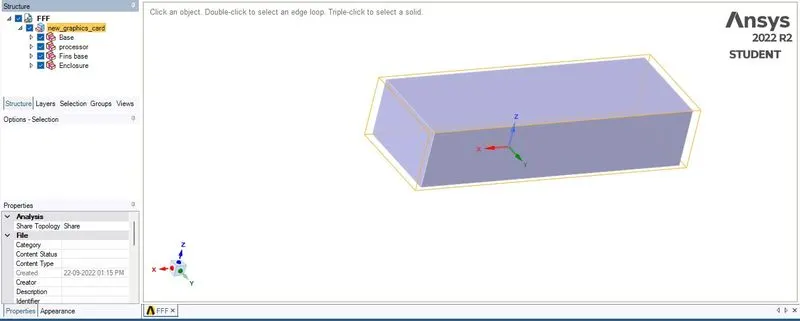
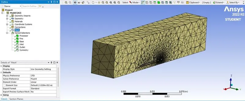
5. Close SpaceClaim and double click on Mesh. Meshing window will appear. Mark Inlet, Outlet, Symmetry, Processor, Fin and Base on geometry by right clicking each part and selecting Create Name Selection. Now select the mesh from the tree and generate mesh with an appropriate element size (0.01mm) to get a base-line meshing on the surface of geometry. The figure shown below represent the geometry after meshing.
6. Close Meshing and double click on Setup, select Double Precision and Fluent window will open. Check all the values and make necessary correction if needed.
7. Select appropriate conditions mentioned below.
Solver - Pressure Based
Viscous - k-epsilon model
Energy - On
Materials - Fluid, Air - Solid , Copper, Silicone, ABS plastic
Note: Properties of Silicone and ABS plastic is taken from the internest sources.
Cell Zone Conditions
Flow region - Fluid - Air
Processor - Solid - Silicone
Fin - Solid - Copper
Base - Solid - ABS plastic
Boundary Conditions
Inlet - Velocity Inlet, Velocity = 1m/s, Temperature = 300K
Symmetry - Symmetry
Outlet - Pressure Outlet
Define surface report with area weighted average of heat transfer coefficient and volume report for maximum temperature.
Solution Initialization - Hybrid Initialization.
8. After assigning all the factors click on Run Calculation and set number of iteration and calculate.
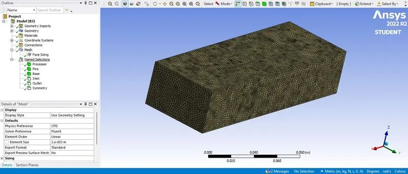
Perform the same simulation with fine meshing In order to create fine meshing on the surface of geometry add Face meshing option and provide the appropriate element size (0.002 mm). The figure shown below represents the geometry with fine meshing.
Note: Run the simulation with different set of inlet velocities and compare the results obtained.
- 1m/sec
- 3m/sec
- 5m/sec
RESULTS AND DISCUSSIONS:
PART-1 - Base-Line Meshing
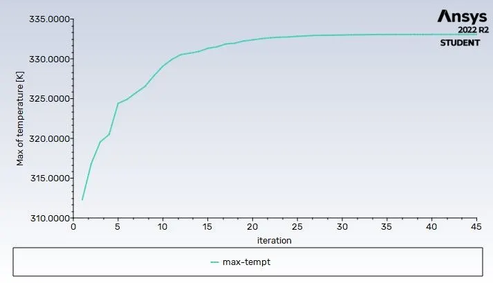
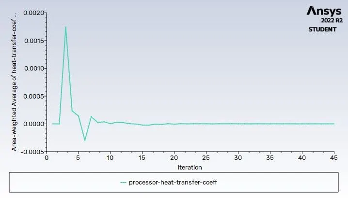
Case - 1 - Inlet Velocity - 1m/sec
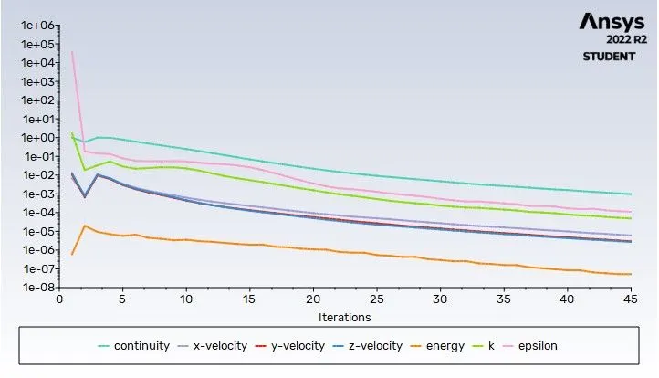
a. Residual Plot
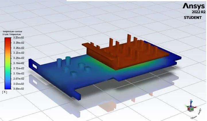
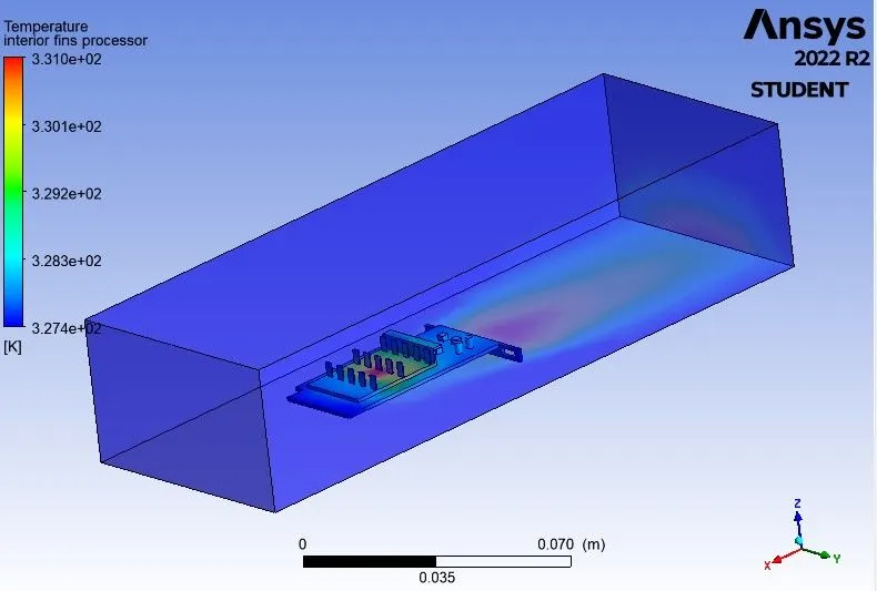
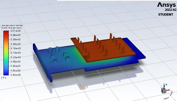
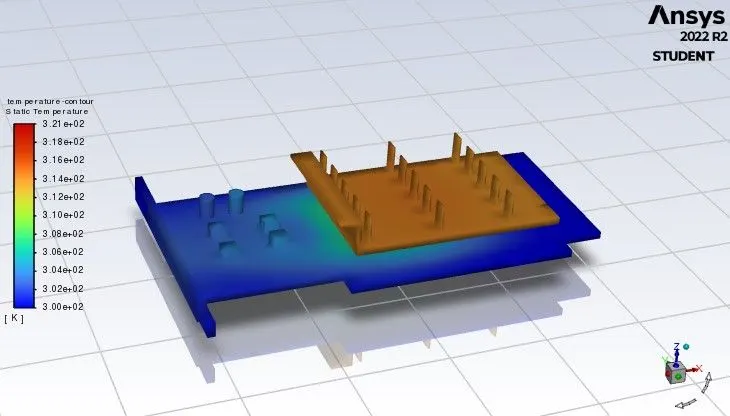
b. Temperature Contour of Graphics Card
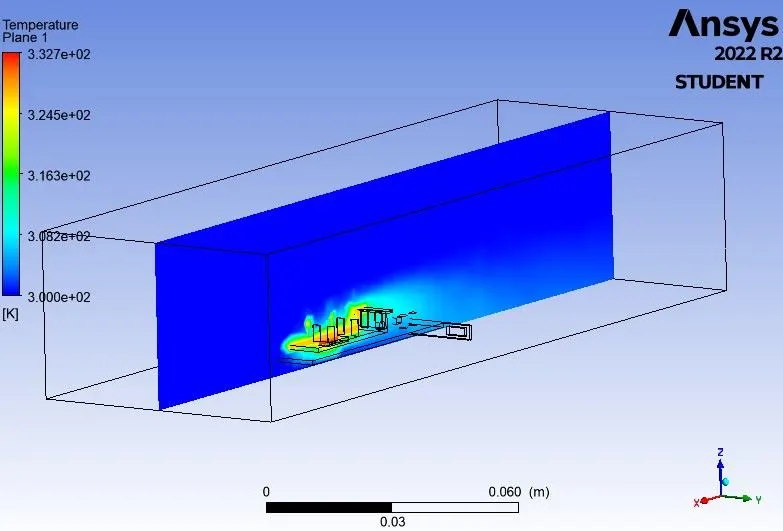
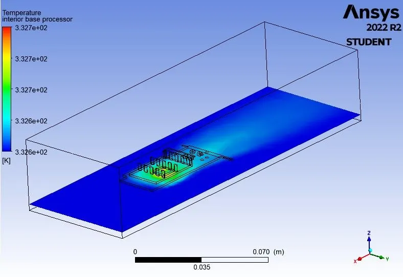
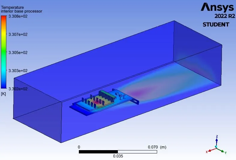
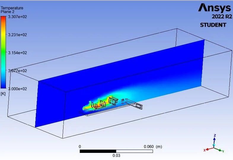
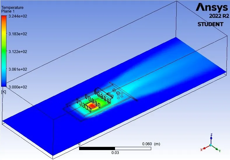
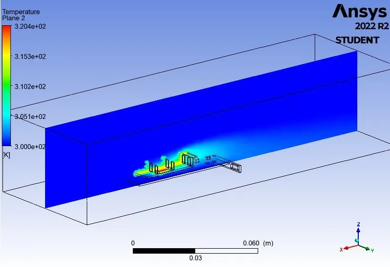
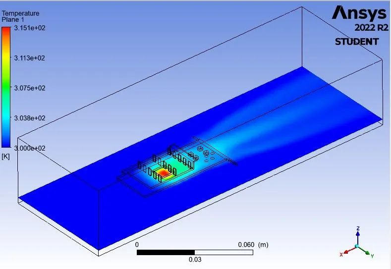
c. Temperature Contour of two planes
d. Maximum Temperature Plot of Processor
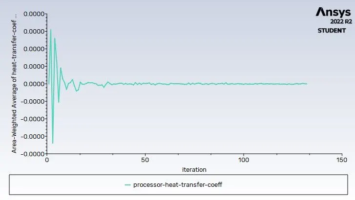
e. Heat Transfer Coeff Plot
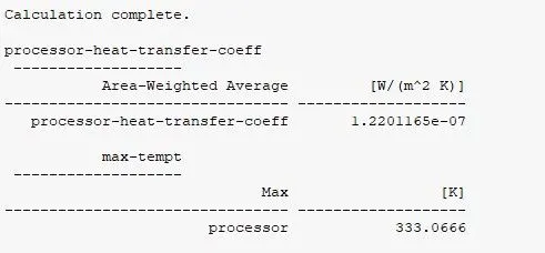
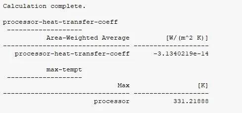
f. Calculated Heat Transfer Coeff and Maximum Temperature
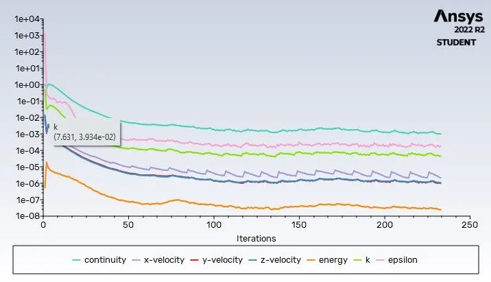
Case - 2 - Inlet Velocity - 3m/sec
a. Residual Plot
b. Temperature Contour of Graphics Card
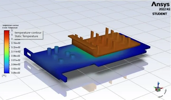
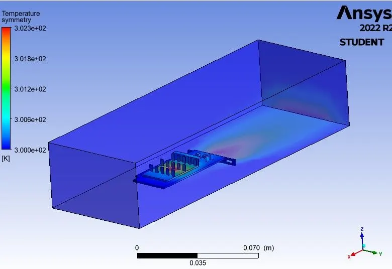
c. Temperature Contour of two planes
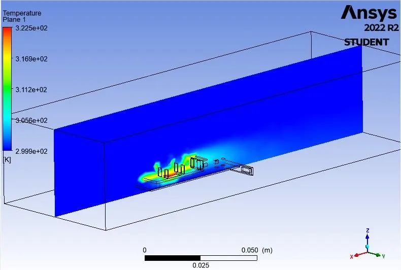
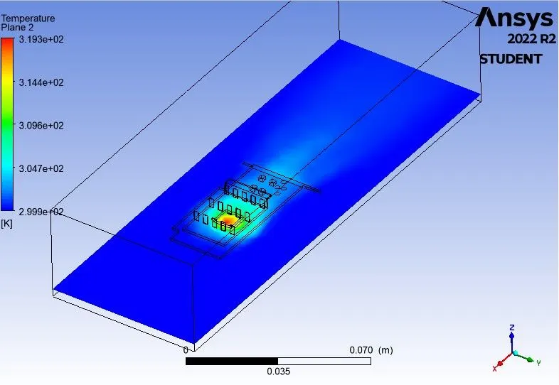
d. Maximum Temperature Plot of Processor
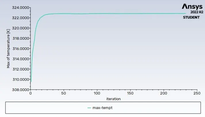
e. Heat Transfer Coeff Plot
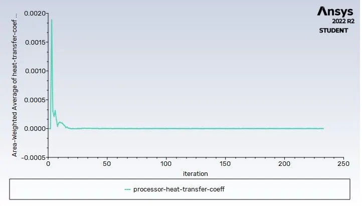
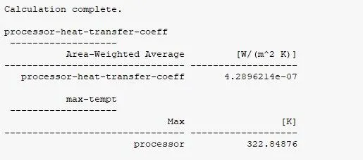
f. Calculated Heat Transfer Coeff and Maximum Temperature
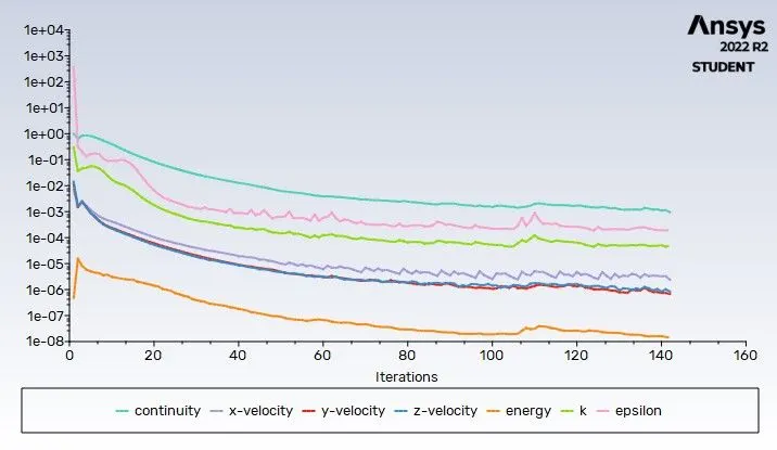
Case - 3 - Inlet Velocity - 5m/sec
a. Residual Plot
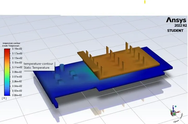
b. Temperature Contour of Graphics Card
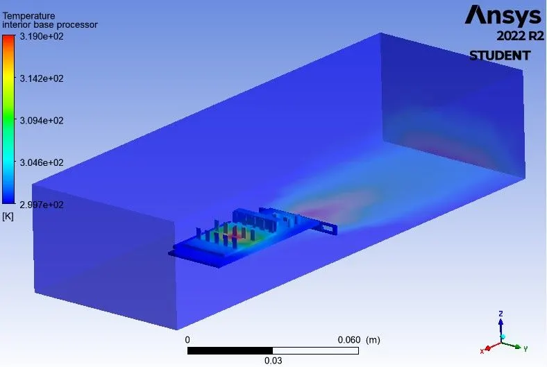
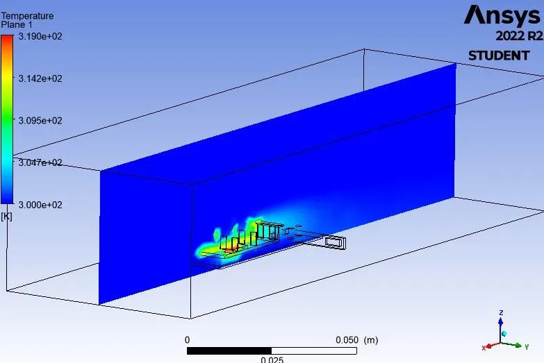
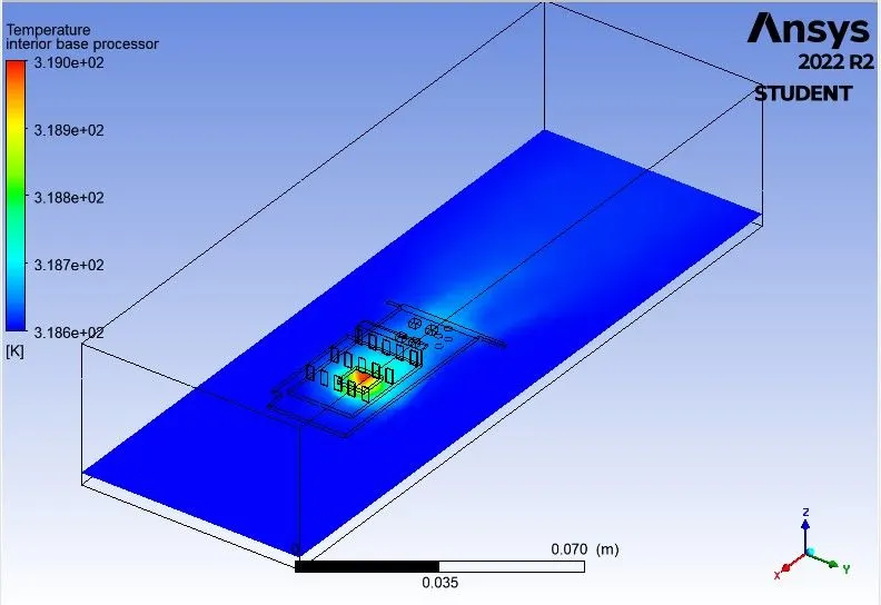
c. Temperature Contour of two planes
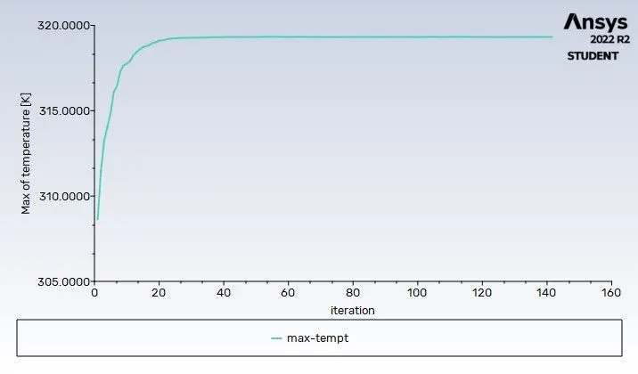
d. Maximum Temperature Plot of Processor
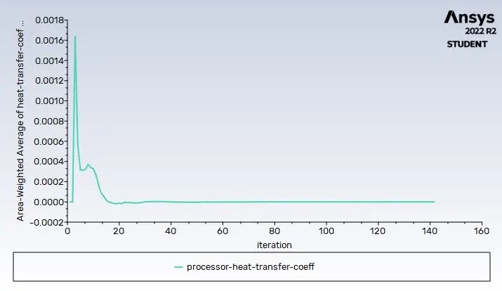
e. Heat Transfer Coeff Plot
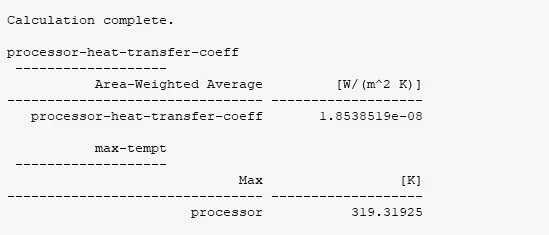
f. Calculated Heat Transfer Coeff and Maximum Temperature
PART-2 - Fine Meshing
Case - 1 - Inlet Velocity - 1m/sec
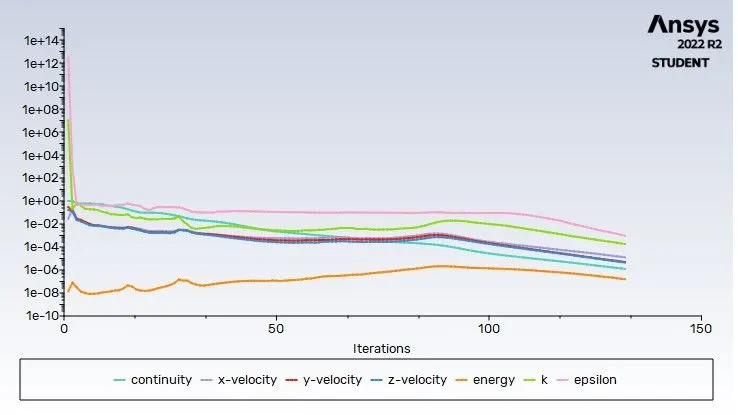
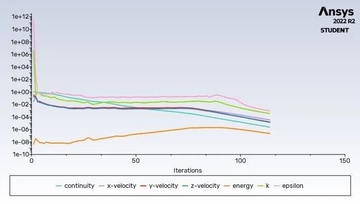
a. Residual Plot
b. Temperature Contour of Graphics Card
c. Temperature Contour of two planes
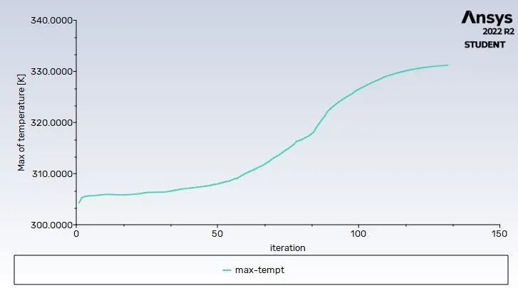
d. Maximum Temperature Plot of Processor
e. Heat Transfer Coeff Plot
f. Calculated Heat Transfer Coeff and Maximum Temperature
Case - 2 - Inlet Velocity - 3m/sec
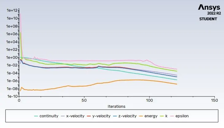
a. Residual Plot
b. Temperature Contour of Graphics Card
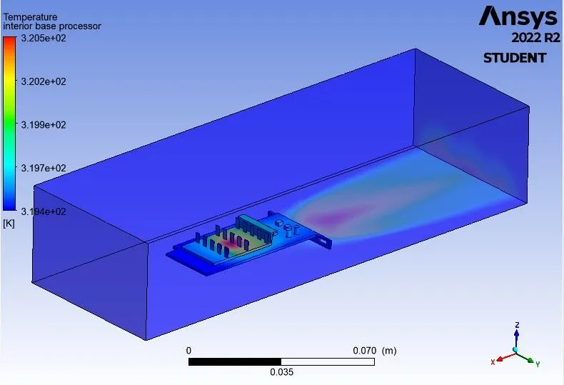
c. Temperature Contour of two planes
d. Maximum Temperature Plot of Processor
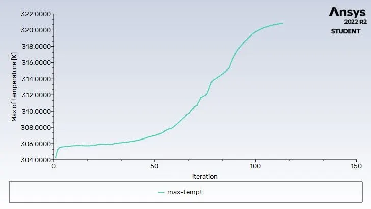
e. Heat Transfer Coeff Plot
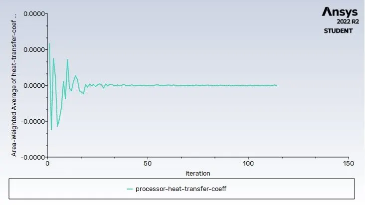
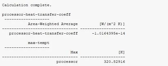
f. Calculated Heat Transfer Coeff and Maximum Temperature
Case - 3 - Inlet Velocity - 5m/sec
a. Residual Plot
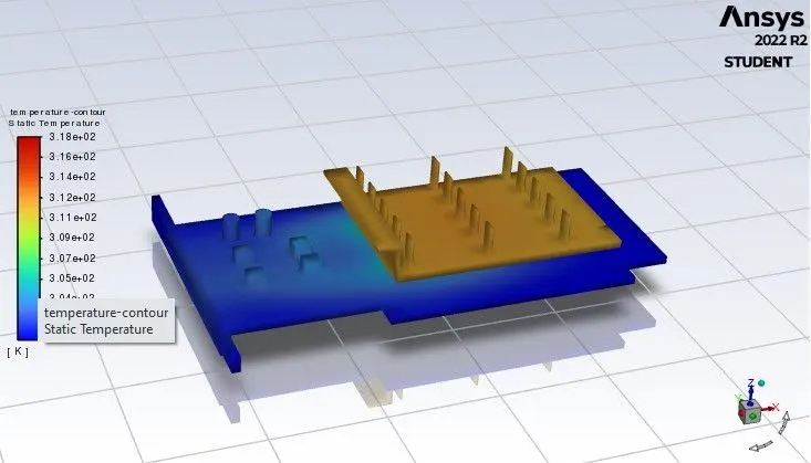
b. Temperature Contour of Graphics Card
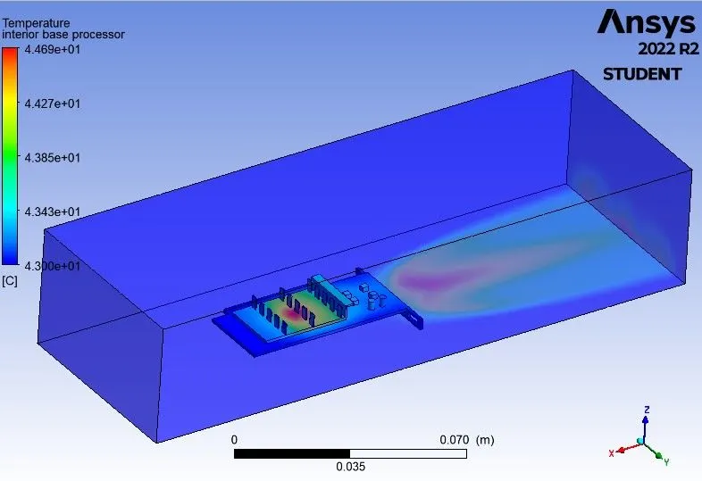
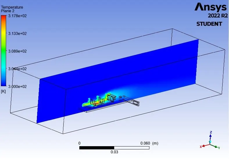
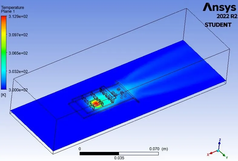
c. Temperature Contour of two planes
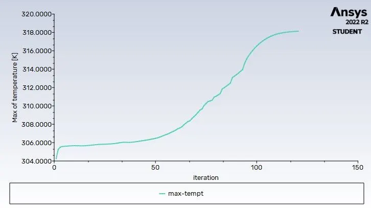
d. Maximum Temperature Plot of Processor
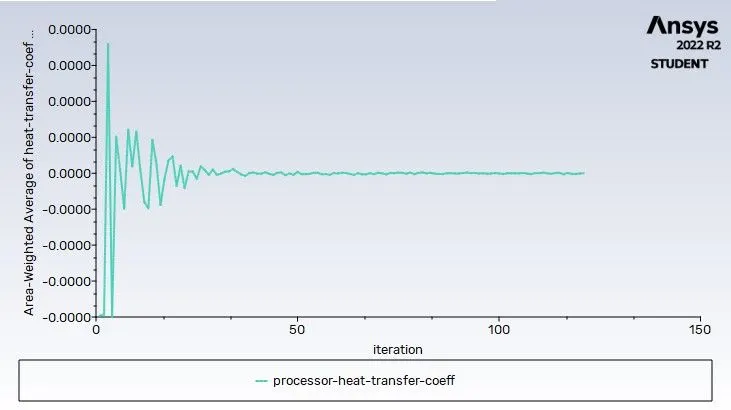
e. Heat Transfer Coeff Plot
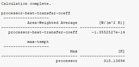
f. Calculated Heat Transfer Coeff and Maximum Temperature
Tables below show the comparison of results obtained from Base-line and fine meshing with different set of cases.
| PART - 1 BASE-LINE MESHING | Cell Counts | Maximum Temperature of Processor | Heat Transfer Coefficient | Iteration at which Solution Converged |
| Case - 1 | 83991 | 333.06 K | 1.22e-07 W/m2.K | 45 |
| Case - 2 | 83991 | 322.84 K | 4.289e-07 W/m2.K | 233 |
| Case - 3 | 83991 | 319.319 K | 1.85e-08 W/m2.K | 140 |
| PART - 1 FINE MESHING | Cell Counts | Maximum Temperature of Processor | Heat Transfer Coefficient | Iteration at which Solution Converged |
| Case - 1 | 301622 | 331.218 K | 3.134e-14 W/m2.K | 132 |
| Case - 2 | 301622 | 320.829 K | 1.016e-14 W/m2.K | 114 |
| Case - 3 | 301622 | 318.136 K | 3.134e-14 W/m2.K | 125 |
From the above tables and figures it is evident that the contours and results obtained are more clear and accurate for fine meshing as compared with baseline meshing. Even though fine meshing take more computational time but the results obtained are accurate. Which can be justified with help of results and contour obtained. It is also concluded that with increase in the inlet velocity maximum temperature of the graphics card decreases.
CONCLUSION:
The simulation of of Conjugate heat transfer analysis on given Graphics card geometry is carried out using Ansys Fluent. From the study it is concluded that the results obtained from part 1 are poor as compared to part 2 as in part 2 fine and high quality meshes are used where as course meshes are in Part -1. Thus the refined mesh allow to produce a clear picture of simulation. The study also gave the idea how the heat transfer and temperature of graphics card are affected with inlet air velocity.