Week 6 - CHT Analysis on a Graphics card
Aim
Conduct a Conjugate Heat Transfer analysis on a model of a graphics card under forced convective airflow at 1, 3 and 5m/s respectively and retrieve the maximum temperature and heat transfer coefficient attained. Further, identify potential hotspots on the model that may be vulnerable to overheating.
Introduction
Conjugate Heat Transfer (CHT) comprises heat transfer in solids, dominated by conduction, and heat transfer in fluids, dominated by convection. The processes are divided into two subdomains and are calculated separately using their respective governing equations. Conditions at the interface of the two are then used to determine the distribution of the temperature/ heat-flux. Conjugate heat transfer analyses are quite often used in HVAC systems, heat sinks, engine cooling, etc.
The optimal working of a graphics card can be achieved when the processor temperature is maintained under a suitable temperature range. The processor will be subject to constant overheating when under heavy load and hence cooling systems are crucial in graphics card design. In the current study, the thermal characteristics of a model graphics card were analysed by subjecting it to various airflow velocities.
Method
Geometry and Fluid Domain
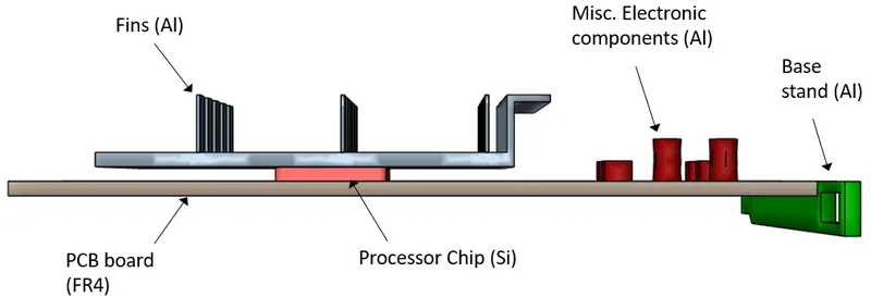
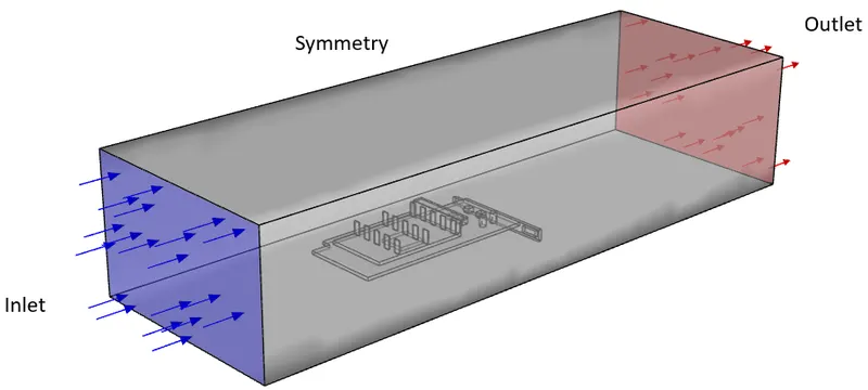
The geometric model of the graphic card and the fluid domain can be seen in the schematic below. The graphics card contains the base PCB board upon which the main processor chip (8mm x 8mm x 1mm) is mounted. This processor chip is cooled by a fins setup placed directly above it. There are also various generic electronic components located on the PCB board along with a stand which will connect the entire graphics card to a desktop casing. The materials used on the graphic card namely Aluminium (Al), Silicon (Si) and glass-reinforced epoxy resin laminate (FR4) are labelled in the schematic shown for their respective components. Details of their material properties are discussed further in the report.
Solver and Boundary Conditions
All simulations were conducted on ANSYS Fluent 2022 R2. The velocity at the flow inlet was changed to 1,3 and 5 m/s for the respective simulations. The pressure outlet at the rear of the domain was set to a 0 gauge pressure relative to the atmosphere. The remaining enclosures of the fluid domain were set to a symmetry boundary condition. A volumetric heat source was applied to the processor chip based on the thermal power output of 1W. This was deemed sufficient for this model as the processor chip is a scaled-down variant. The resulting volumetric heat generation rate applied to the processor chip was 1.5625e+7 W/`m^3`.
The materials and their properties used in the analysis are tabulated below [1]:
| Material | Zone |
Density [kg/`m^3`] |
Specific Heat Capacity [J/kg.K] |
Thermal Conductivity [W/m.K] |
Viscosity [Kg/m.s] |
| Air | Fluid | 1.225 | 1006.43 | 0.0242 | 1.7894e-05 |
| Aluminium (Al) | Solid | 2719 | 871 | 202.4 | - |
| FR4 | Solid | 1850 | 1150 | 0.294 | - |
| Silicon (Si) | Solid | 2329 | 710 | 149 | - |
The steady-state pressured-based PV coupled scheme was used to discretize the flow parameters. The energy equation was enabled for this analysis. Turbulence in the flow was predicted using the two-equation K-Omega SST model. The second order scheme was used to estimate the pressure, the second order upwind scheme was used to estimate momentum and energy and the first order upwind scheme was used to estimate the turbulence parameters. The solution was initialized by hybrid initialization followed by an FMG initialization to quicken the simulation. The simulation was run with pseudo transient time stepping with an automatic global conservative length scale. Convergence was checked by the scaled residuals to reach 1e-3 and the variations in the maximum temperature on the processor chip and maximum surface heat transfer coefficient on the processor chip not exceeding 1e-3 units across iterations. Simulations typically took under 200 iterations to achieve convergence.
Mesh Generation and sensitivity analysis
An initial baseline mesh was generated with coarse sizings to understand the flow field and hotspots on the model. Using the results from the baseline simulation, refinements of the mesh were focused on the fins of the graphics card as those bodies were seen to contribute to the main source of cooling/ heat transfer. The image below shows the surface mesh on the baseline (left) and refined mesh (right) respectively.
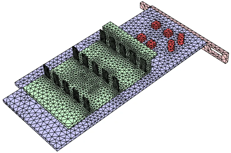
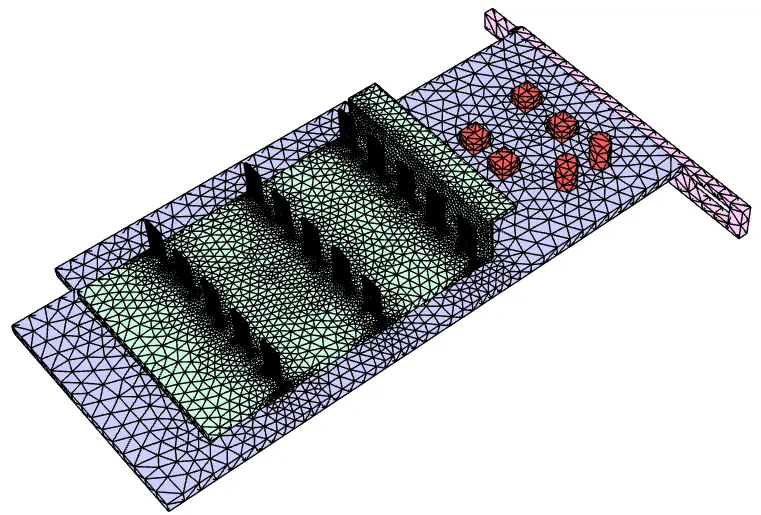
As seen above, the base PCB board, electronic components and the stand were maintained coarse in the refined mesh as they did not contribute much to the heat transfer on the processor chip. Inflation layers were unchanged in the baseline and refined case and were calculated to ensure the first layer was within the viscous sublayer of the boundary layer. This resulted in four inflations layers generated with a Smooth Transition of 0.4 in the fluid domain and two inflations layers generated with a first layer height of 2e-4 m in the solid domain. The wall `y^+` for the 5m/s case can be seen in the image below with the highest wall `y^+`< 5.
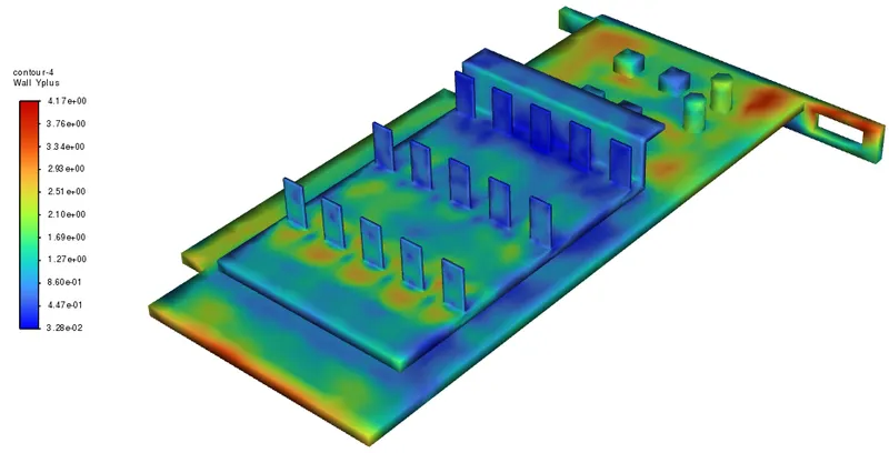
The details of the mesh sizing are tabulated below:
| Mesh | Mesh Size | Fins- Face Sizing | Fins - Edge Sizing | Fins- Plate Face Sizing | Processor - Body Sizing | Misc Electronics- Sizing | PCB Board/ Stand - Sizing |
| Baseline | 258K | 4.5e-4 m | - | 1.5e-3 m | 5e-4 m | 1e-3 m | 1.5e-3 m |
| Refined | 511K | 8e-4 m | 2e-4 m | 1e-3 m | 5e-4 m | 1e-3 m | 1.5e-3 m |
The sensitivity analysis was performed on the 5m/s case as it had the highest flow velocity and therefore highest heat transfer through convection. The image below shows the convective heat transfer coefficient distribution over the fins on the baseline (left) and refined mesh (right) respectively.
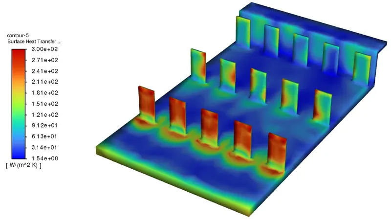
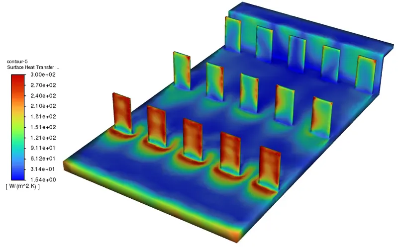
The baseline mesh is able to capture the overall distribution of the heat transfer coefficient well however, the refined mesh provides more clarity of its distribution on the fins and around it. Since the major source of convective heat transfer is done on the fins, the refined mesh was deemed appropriate to perform all simulations in the analysis.
Results
The images below show the development of the scaled residuals of the simulations across iterations. It can be seen that cases 2 and 3 have reached 1e-3 but however case 1 has struggled to do so and had stabilised at approximately 5e-3. Ensuring convergence in the cases need to be further checked by monitoring additional parameters in the model.
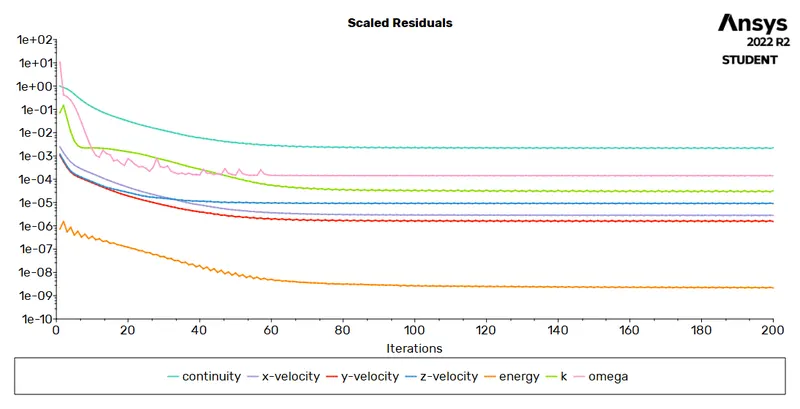
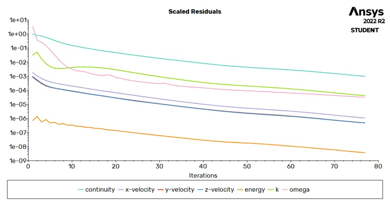
Case 1: 1m/s Case 2: 3m/s
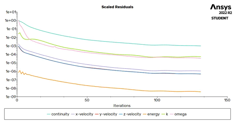
Case 3: 5m/s
The images below show the variations in the maximum temperature on the model across iterations. All cases are seen to stabilise on a particular value and this is an indication that the flow has reached a steady state.
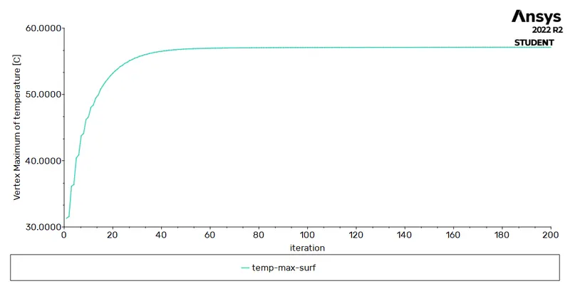
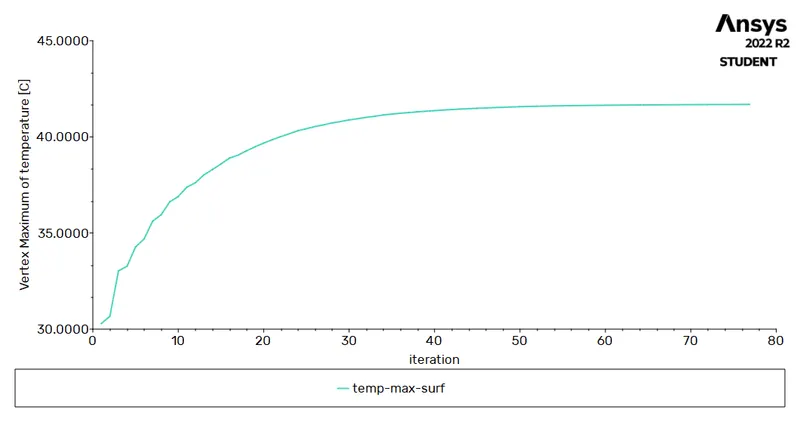
Case 1: 1m/s Case 2: 3m/s
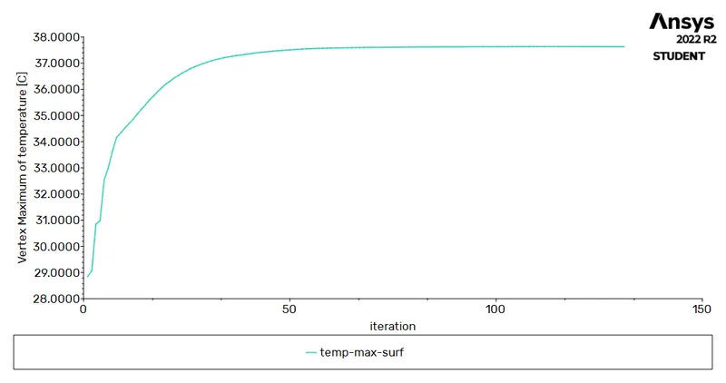
Case 3: 5m/s
The images below show the variations in the maximum convective heat transfer coefficient on the processor across iterations. All cases are seen to stabilise on a particular value and this is an indication that the flow has reached a steady state.
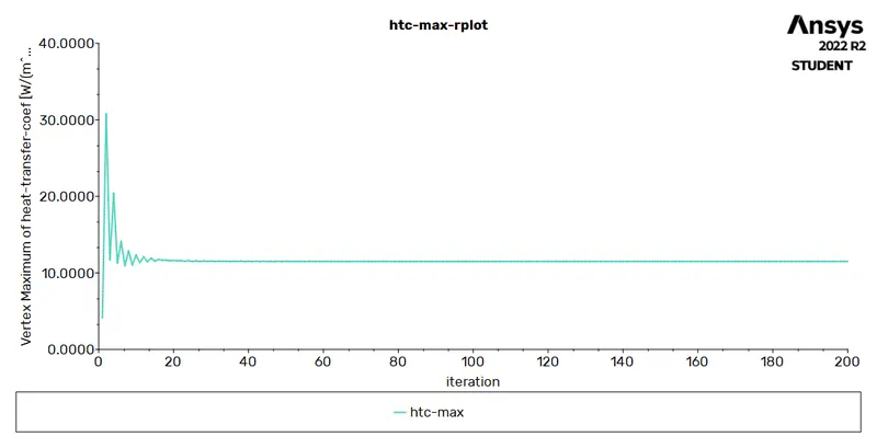
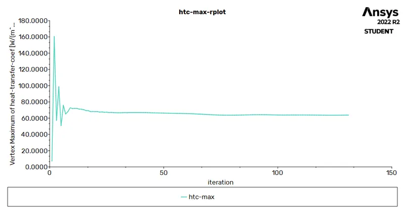
Case 1: 1m/s Case 2: 3m/s
Case 3: 5m/s
With the above figures of the scaled residuals, maximum temperature and max heat transfer coefficient plots, the solution results of the respective simulations can thus be deemed converged.
The images below show the temperature on the fins setup mounted on the graphic card and the pathlines of airflow around it for the different cases. Case 1 shows the highest temperature recorded on the fins and it also has the lowest air velocity of 1 m/s. Case 2 shows an immediate drop in temperature with an air velocity of 3m/s and case 3 shows the lowest max temperature on the model as it has the highest air velocity of 5m/s. This peak in temperature in case 1 and the gradual decrease of the max temperature in the consecutive cases can be attributed to the amount of convective heat transfer done on the model. This convective heat transfer depends directly on the airflow velocity and thus is reflected in the results of the simulation.
The flow field around the model is seen to be similar across the cases with stagnation at the first set of fins and air recirculation behind it. This stagnation of the flow causes the air to lose its velocity and thus the second and third row set of fins show a higher temperature on them compared to the first. This result is consistent in all cases and therefore decreasing the region of stagnation is crucial to the cooling on the graphics card which may be done by a change in the fins design or setup.
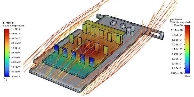
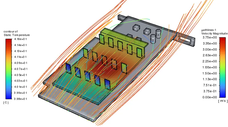
Case 1: 1m/s Case 2: 3m/s
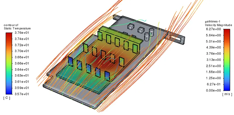
Case 3: 5m/s
The images below show the temperature distribution on the graphics card without the fins, to visualise the cooling from the fins. Case 1 shows the maximum temperature achieved on the processor chip and also shows the largest area of temperature distribution on the PCB board. Case 2 shows the immediate drop in temperature and reduction in the area of increased temperature on the PCB board followed by case 3 with the least max temperature and least area of increased temperature on the PCB board. These results are consistent with previous images showing the temperature distribution on the fins and thus show the importance of the fins set up in the cooling of the graphics card.
The temperature distribution upstream of the processor is seen to be lower compared to the regions downstream. This is due to the reduction in air velocity in those regions as the flow field is subjected to stagnation by various obstacles which lead to recirculation and hence loss in flow velocity. The PCB board is seen to have a lower temperature overall compared to the other components on the graphics card, this can be attributed to the FR4 material having a very low thermal conductivity.
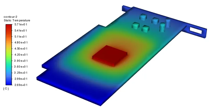
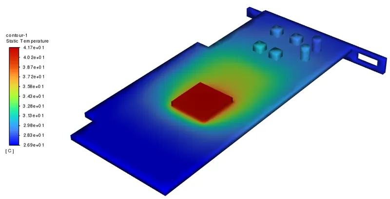
Case 1: 1m/s Case 2: 3m/s
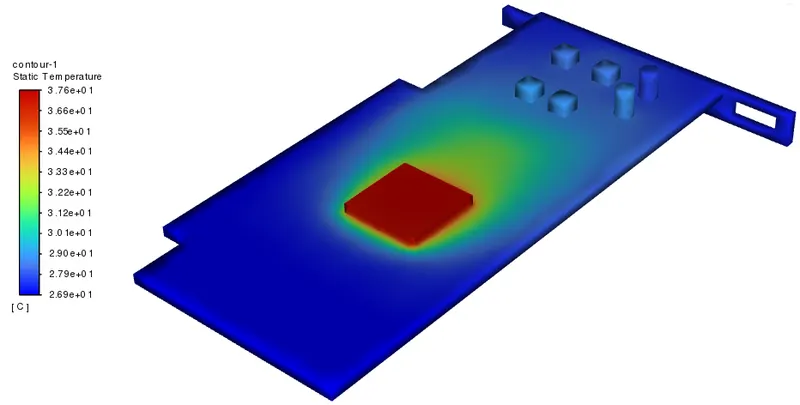
Case 3: 5m/s
The final results of the max temperature and the max heat transfer coefficient on the processor chip are tabulated below:
| Case id | Max Temperature [C] | Max Heat Transfer Coefficient [W/`m^2` K] |
| Case 1 : 1m/s | 57.26 | 11.5 |
| Case 2 : 3m/s | 41.94 | 32.35 |
| Case 3 : 5m/s | 37.77 | 63.81 |
The table is coherent with the qualitative analysis done using the temperature and velocity distributions above and clearly shows the importance of air flow velocity on the cooling of the graphics card.
Conclusion
A conjugate heat transfer analysis was performed on the given graphics card model with varying flow velocities of 1m/s, 3m/s and 5m/s. A qualitative analysis was performed using the temperature distributions and flow field pathlines to visualise the nature of the cooling on the graphics card. The max temperature and the max heat transfer coefficient have also been tabulated and directly reflect the results of the qualitative analysis. From the simulations, it was evident that increasing the airflow velocity has brought about an increased cooling performance on the graphics card. It was also noted that the current setup of fins created a large stagnation region behind the first stage of fins making the second and third stage fins work inefficiently. This needs to be minimised by modifying the design of the fins to achieve an efficient and increased cooling performance.
References
- Thermal Properties of Non-Metals, Engineers Edge:
https://www.engineersedge.com/heat_transfer/thermal_properties_of_nonmetals_13967.htm