1. Introduction

The Objective is to perform a Conjugate Heat Transfer Analysis in Graphics Card and to monitor the effect of velocity (Reynolds Number) on the heat transfer.

2. Problem Statement

1. Run the simulation by varying the velocity from 1m/sec to 5m/sec for at least 3 velocities and discuss the results.
2. Find out the maximum temperature and heat transfer coefficient attained by the processor.
3. Prove that the simulation has achieved convergence with appropriate images and plots.
4. Identify potential hotspots on the model.

The data inputs that have been assumed for solving this problem are,

Data Input:

1. Processor - Silicon (Default Values)
2. Heatsink and Capacitors - Aluminum (Default Values)
3. Rest of the Graphics Card - FR4(Values shown in next section) [This material is used in current graphic cards]
4. Fluid - Air (Default Values)

Heat Generation in Processor:

1. Power = 5W (Assumed)
2. Area = 64m³
3. Heat Generation Rate = power/Area = 78125000 W/m³

Inlet velocity:

1. First Case - 5 m/s
2. Second Case - 4 m/s
3. Third Case - 3 m/s
4. Fourth Case - 2 m/s
5. Fifth Case - 1 m/s

3. Problem Setup for Simulation

3.1 Geometry Setup

1. The Geometric model is received into SpaceClaim has been prepared for simulation by performing shared topology which is necessity for Conjugate Heat Transfer analysis.
   
   
   
   
   
   
   
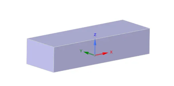
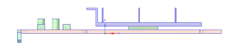
2. It is necessary to make sure that the Topology of the Geometry is Shared.
   
   

3.2 Mesh Setup

1. For this particular case mesh must be refined for the processor and the sink for better Temperature field values so the mesh is considered to be 0.2 mm of element size for the enclosure and 1mm, 0.4mm and 1 mm for the Heat Sink, Processor and the Capacitors Respectively. Also find the Mesh Element Quality for the same.
   
   
   
   
   
   
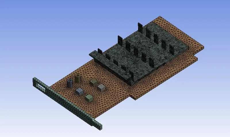
2. The Named Sections are given accordingly.

3.3 Solver Setup

1. For Steady State simulation, Steady is selected in the Time Section of the General Tab is to be selected.
   
   
   
   
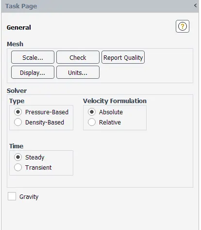
2. “K-Epsilon” is used in the Viscous Tab. In the Create Materials section, “FR4” is to be created into the material section and the rest of the elements mentioned above can be copied from the Fluent Database.
   
   
   
   
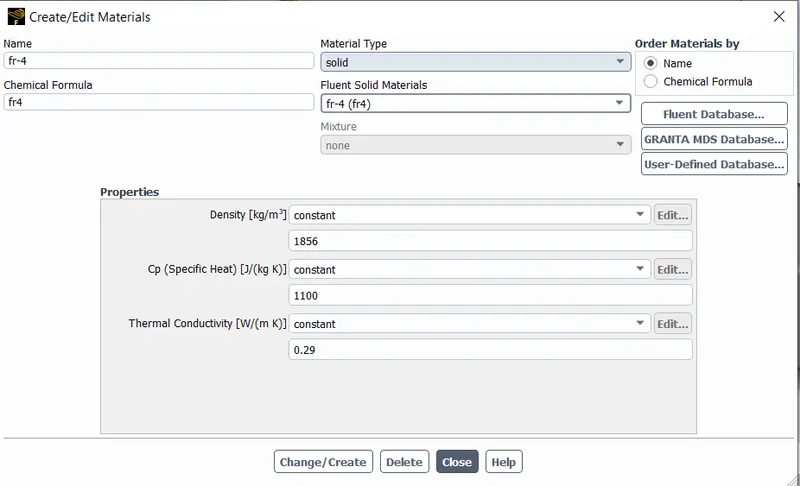
3. For Energy assign one and a window will pop up and give a value of 7,81,25,000
4. The Area Weighted Average Reports are to be defined from the Definitions for the Processor Temperature and Heat transfer Coefficient for the same.
5. Number of Iterations is set to 300 and the calculation is run.

4. Simulation Results

4.1 Case – 1: Velocity as 5 m/s

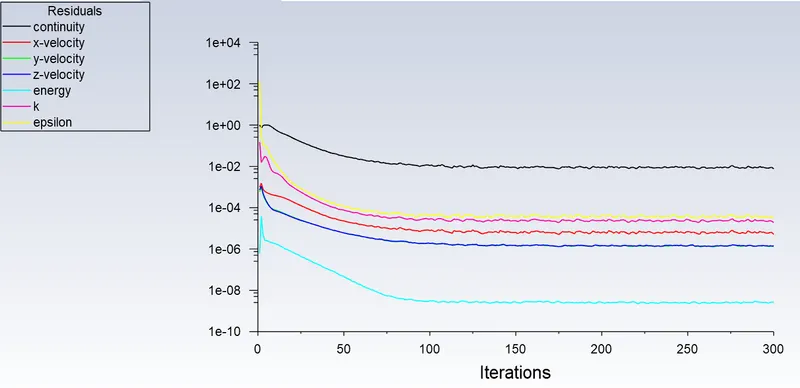
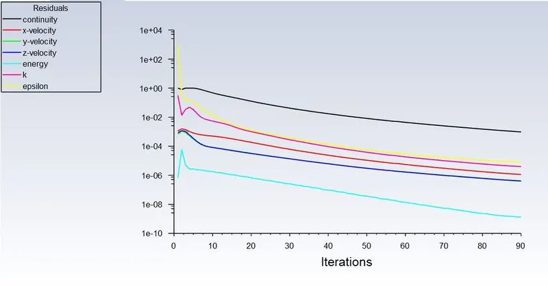
1. Residual Scaled Graphs
   
   
   
   
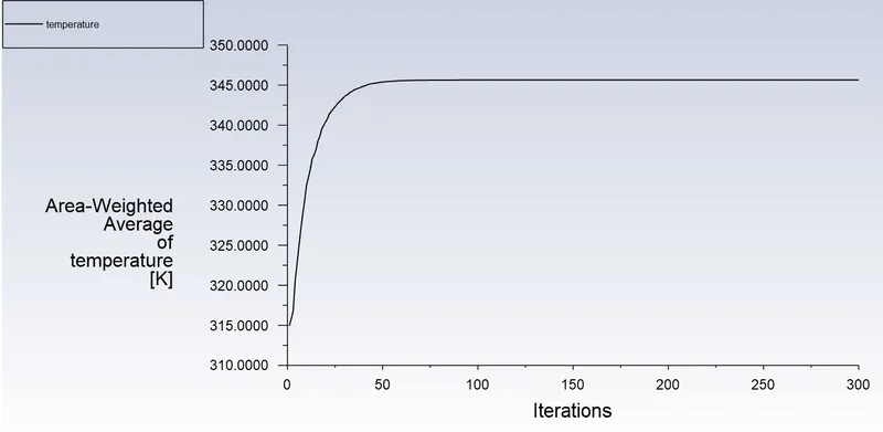
2. Area Weighted Average of Temperature
   
   
   
   
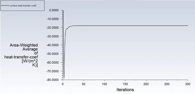
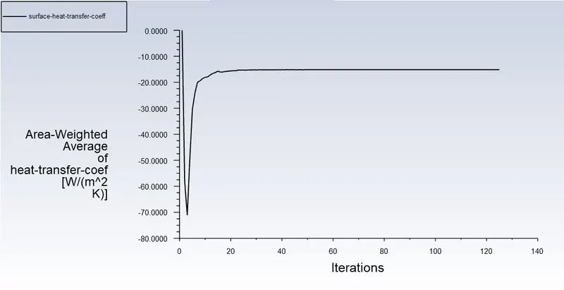
3. Area Weighted Average of Heat Transfer Coefficient
   
   
   
   
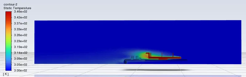
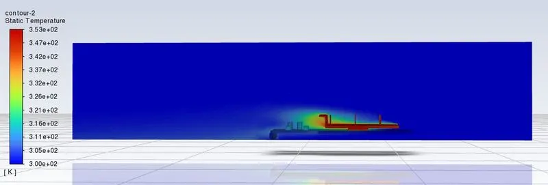
4. Temperature Contour for Fluid Flow
   
   
   
   
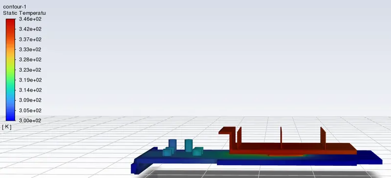
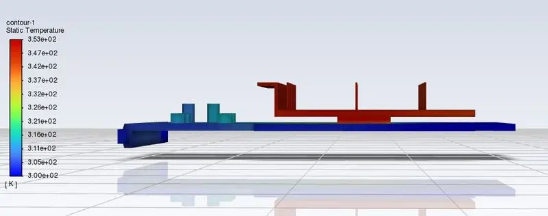
5. Temperature Contour for Graphic Card
   
   

4.2 Case – 2: Velocity as 4 m/s

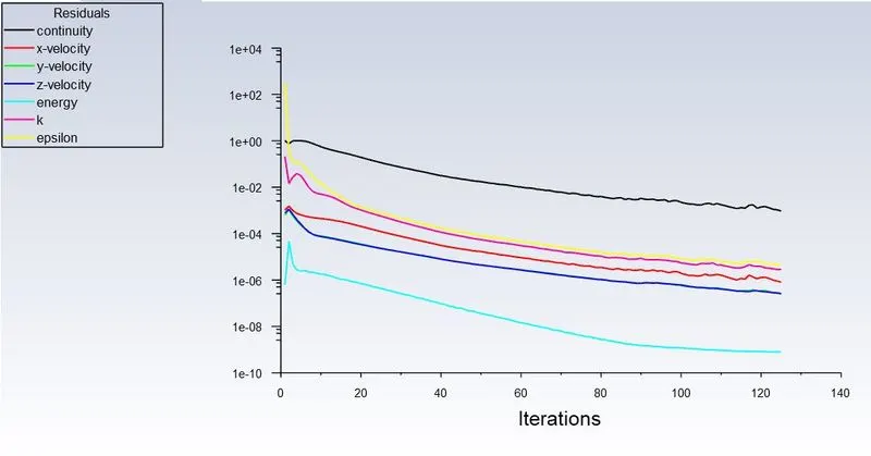
1. Residual Scaled Graphs
   
   
   
   
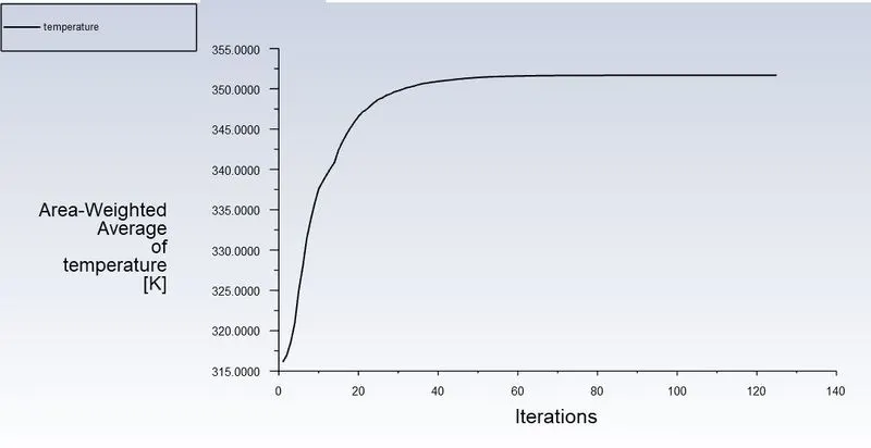
2. Area Weighted Average of Temperature
   
   
   
   
3. Area Weighted Average of Heat Transfer Coefficient
   
   
   
   
4. Temperature Contour for Fluid Flow
   
   
   
   
5. Temperature Contour for Graphic Card
   
   

4.3 Case – 3: Velocity as 3 m/s

1. Residual Scaled Graphs
   
   
   
   
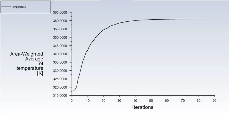
2. Area Weighted Average for Temperature
   
   
   
   
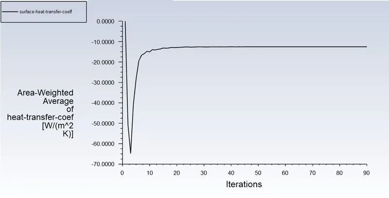
3. Area Weighted Average for Heat Transfer Coefficient
   
   
   
   
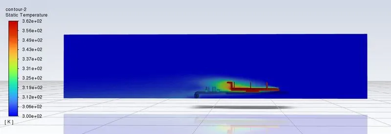
4. Temperature Contour for Fluid Flow
   
   
   
   
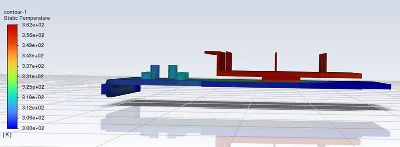
5. Temperature Contour for Graphic Card
   
   

4.4 Case – 4: Velocity as 2 m/s

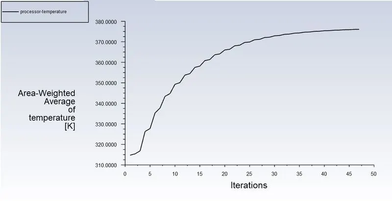
1. Area Weighted Average for Temperature
   
   
   
   
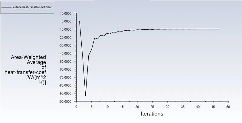
2. Area Weighted Average of Heat Transfer Coefficient
   
   
   
   
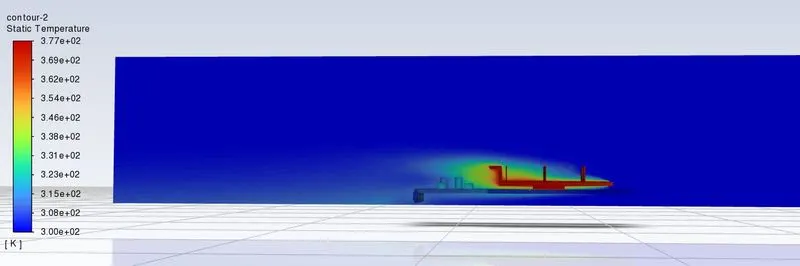
3. Temperature Contour for Fluid Flow
   
   
   
   
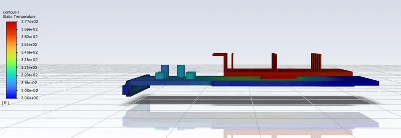
4. Temperature Contour for Graphic Card
   
   

4.5 Case – 5: Velocity as 1 m/s

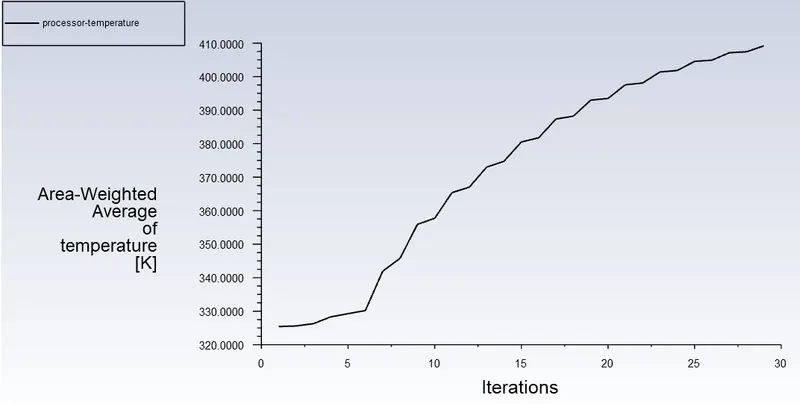
1. Average Weighted Area for Temperature
   
   
   
   
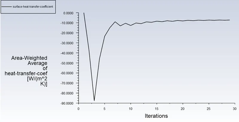
2. Area Weighted Average of Heat Transfer Coefficient
   
   
   
   
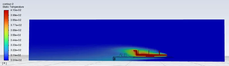
3. Temperature Contour for Fluid Flow
   
   
   
   
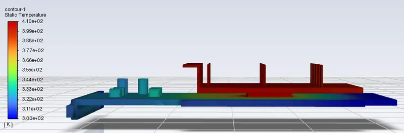
4. Temperature Contour for Graphic Card
   
   

5. Discussion of Results and Conclusion

Flow Velocity (m/s)	Maximum Temperature (K)	Heat Transfer Coefficient (W/m2.K)
5	346	-18.2638
4	353	-15.3526
3	362	-12.3256
2	377	-10.7741
1	410	-8.1632

From above table of Temperatures and coefficients for all the cases, it can be observed that the maximum temperature of processor increases with a decrease in velocity of air flow and heat transfer coefficient was almost similar for 5 m/s & 3 m/s air flow velocity case, but for 1 m/s, heat transfer coefficient has been decreased drastically & similar phenomena also can be seen in maximum temperature values as well.

Convergence:
The convergence for a simulation can be achieved when the errors either fall consistently or when the residuals seem to repeat through the execution of iterations where it can be decided as converged. This can be observed through out the above Residual Scaled Graph for each case for 5 m/s to 1 m/s velocities.

From the above Temperature Contours for Graphic Card, it can be observed that the Heatsink and the Processor has the highest temperature when compared to any other region or the components. It is observable that the heat distribution takes place from Processor to the Heatsink as the Heat generation takes place at the Processor. So, these are considered to be Hot Spots.