1. Introduction

1.1 Rayleigh Taylor Instability

The Rayleigh Taylor Instability is the interference between fluids of different densities. In general, it can be observed majorly between High density and Low-density Liquids for higher density liquid being at the bottom and the Lower density liquid on the top.

This instability can be observed when the high-density liquid starts interference with the low-density liquid. For a regular example, considering a container of oil, when water is poured into it, water starts to flow downwards to the bottom of the container with respect to the gravity. This disturbance of the high-density fluid flowing through low-density fluid causes the potential energy to increase for it and the fluid with lesser density displaces upwards.

In terms of analysing this Instability, the displacement of fluid can be approximated equations and its amplitude of perturbation with respect to time.

1.2 CFD Models based on mathematical analysis of Rayleigh Taylor Waves

1. Kevin-Helmholtz (KH) Instability – It is the instability that occurs between the fluids which does not form a homogenous mixture with a velocity differential for their interface. The creation of small-scale motion at the interface defines these patterns. It ultimately results in the development of an unstable vortex street at the interference. Spiral streams are produced as a result at the interface layer of the fluids.
2. Plateau-Rayleigh Instability - It describes why and how a jet of fluid falling to the interface layer of the other fluid fragments into smaller packets that have the same volume but less surface area. This Instability is fueled by the tendency of liquids to have smaller surface areas due to their surface tensions.
3. Richtmyer - Meshkov Instability (RMI) - It happens when two fluids with differing densities accelerate abruptly as a result of a shock wave. Slowly varying disturbances that first increase at constant rate are the beginning stages of the instability's progression. Then comes a nonlinear domain, in which bubbles form when a lighter fluid flow penetrates a heavy fluid and spikes form when a denser fluid penetrates a lighter fluid. These fluids finally combine as a chaotic regime. This instability may be thought of as the Rayleigh-Taylor instability's impulsive-acceleration limit.

1.3 Atwood Number

The Atwood number (A) is a dimensionless number in fluid dynamics used in the study of hydrodynamic instabilities in density stratified flows.

`Atwo od Number (A)=(ρ_1-ρ_2)/(ρ_1+ρ_2 )`

Where,

ρ₁ = Density of the Heavier Fluid

ρ₂ = Density of the Lighter Fluid

Understanding the distance at which heavy fluid bubbles penetrate light fluid, which is a function of acceleration time scale, is helpful.

So, by calculating the Atwood Number for the above cases,

2. Problem Statement

The problem is about simulating the flow over a cylinder for both Steady State and Unsteady State conditions by varying the Reynolds Number (Re) as mentioned below to understand the Vortex Shedding effects in the flow. This objective is needed to be achieved using Fluent Solver. The Flow simulation is to be performed for the Reynolds Numbers (Re) in the first part of the assignment with,

3. Problem Setup for Simulation

3.1 Geometry Setup

1. A square is drawn of the dimensions 20mm x 20mm which is pulled to create a surface using Pull tool. This component is named Air.
2. Another square is drawn above the Air component of the dimensions 20mm x 20mm which is pulled to create a surface using Pull tool. This component is named Water.
   
   
   
   
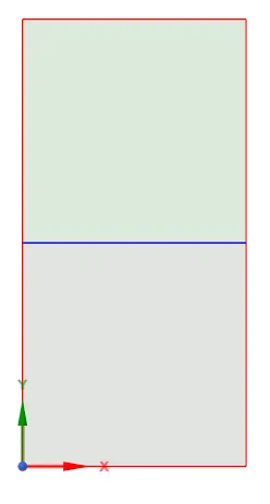
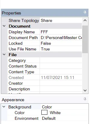
3. The topology of the created components needs to be Shared in-order to create the interference between these fluid components. For this, the Share tool needs to be utilised and to be made sure that the topologies are shared.
   
   

3.2 Mesh Setup

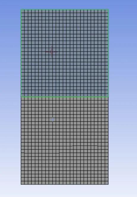
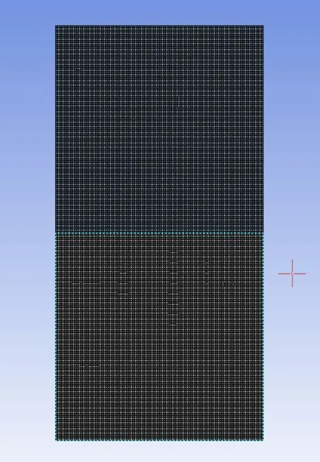
1. The Element size for the first case is set to default but coming to the first case the element size is set to 0.8 mm and for the second case, it is set to 0.2 mm. This is as represented below where, image on the left being 0.8 Mesh and image on the right being 0.2 Mesh
   
   

3.3 Solver Setup

1. For Steady State simulation, Steady is selected in the Time Section of the General Tab is to be selected.
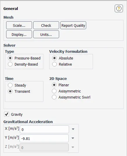
2. Since the instability needs to be captured, 'Transient' is selected from General Tab and Gravity is enabled for this as the high-density fluid is setup on the top.
   
   
   
   
3. “Laminar” is Viscous Tab. In the Create Materials section, “water-liquid” is to be copied into the material section.
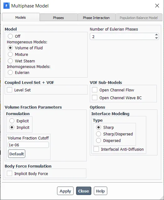
4. In the Multiphase section. Implicit method is selected and in the Phases section, Name = air; Phase Material = air, Name = water; Phase Material = Water is selected as per the problem statement.
   
   
   
   
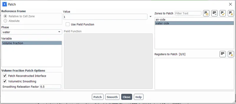
5. A Standard Initialisation for this case and after that, in the “Patch”, Water is assigned the value of 1 and patch and Air assign value of 0 and patch. Time Step size = 0.005 s.
   
   
   
   
6. Number of Time Step is set to 500 and the calculation is run.

4. Simulation Results

4.1 Case – 1: Default Fluid

1. Mesh of 0.8 mm
   
   
   
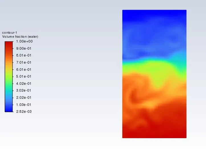
   Video Link: Simulation for Mesh of 0.8 mm
   
   
2. Mesh of 0.2 mm
   
   
   
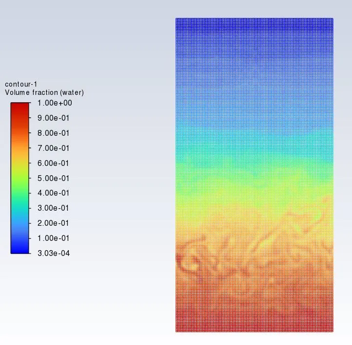
   Video Link: Simulation for Mesh of 0.2 mm

4.2 Case – 2: User Defined Fluid

1. For a Viscosity of
   
   
   
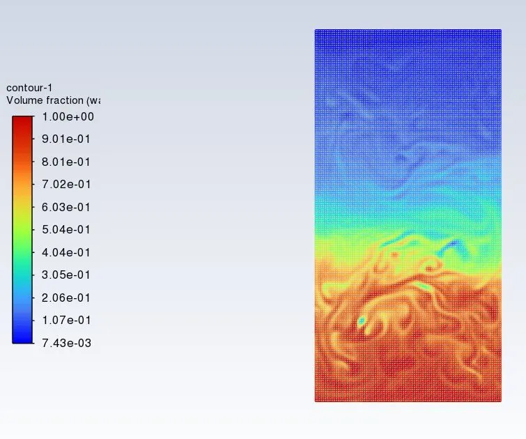
   Video Link: Simulation for Mesh of 0.2 mm with User Defined Material

5. Discussion of Results and Conclusion

For the above cases, the Atwood Number can be calculated from the formulae mentioned in the first section.

ρ₁ = 998.2 kg/m³ ; ρ₂ = 1.225 kg/m³ for Water (H₂O Liquid)

ρ₁ = 998.2 kg/m³ ; ρ₂ = 400 kg/m³ for User defined Material

1. For Case 1:
   
   Atwood Number = (998.2 - 1.225) / (998.2 + 1.225) = 0.9975
   
   
2. For Case 2:
   
   Atwood Number = (998.2 - 400) / (998.2 + 400) = 0.4278

From above calculation for both the cases, it is clear that first case has achieved the stability after setting up the instability conditions but in case of second simulation, the flow became unstable and get back to its original states by taking considerable amount of time meaning it is an unstable flow. It also can be observed the from the above results that as the higher mesh resolution are utilised, the solution becomes unstable but at the same time the it helps in capturing the flow patterns accurately.

There are more bubbles and spikes in the first case (coarse and refine) case when compared to third case, because the density difference is less, therefore the Atwood number is low and the penetration is also low for the third case.