Calculating the Stretch Ratio and comparing the ELFORM (-2,-1,1,2) with Ogden_Material Model by plotting the stress vs stretch ratio curves.
OBJECTIVE:
- To Create a block of 10mmx10mmx10mm dimension with 10 elements for each direction and use the material card attached (Ogden_Material.k)
- Use appropriate boundary conditions to simulate tensile behavior for the model and finally compare the results from your simulation to the plot above up to stretch ratio 5. Only the uniaxial plot is to be compared.
- Compare the results for the simulation using ELFORM = 1, 2, -1, -2
- The unit of µ in the material definition is in MPa and α is a dimensionless quantity. Modify those quantities according to your unit systems.
- Use a proper solver (Implicit/Explicit) and also explain the reason.
PROCEDURE:
- Creating the FEA model
- Open LSPP. Create a box using solid Hexa elements as such that the dimensions are 10*10*10 with 10 elements in each direction. This can be done using the Shape mesher option under the Mesh panel.
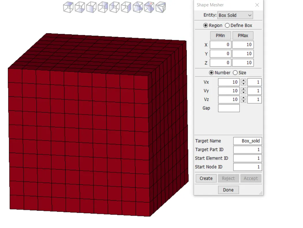
Figure.1.Creating the box with required dimensions
- Define a *SECTION_SOLID card and set the Eleform as 1. and assign the section card to the box created. Note: In this assignment, we need to run the same simulation with different elforms, -1,-2,1, and 2. Thus change the elform in the keyword file for each case separately and save it for each case before running the analysis.
Elform = 1:Constant stress solid element: default element type
Elform = -1: Fully integrated S/R solid intended for elements with poor aspect ratio, efficient formulation
Elform = 2: Fully integrated S/R solid
Elform = -2: Fully integrated S/R solid intended for elements with poor aspect ratio, accurate formulation
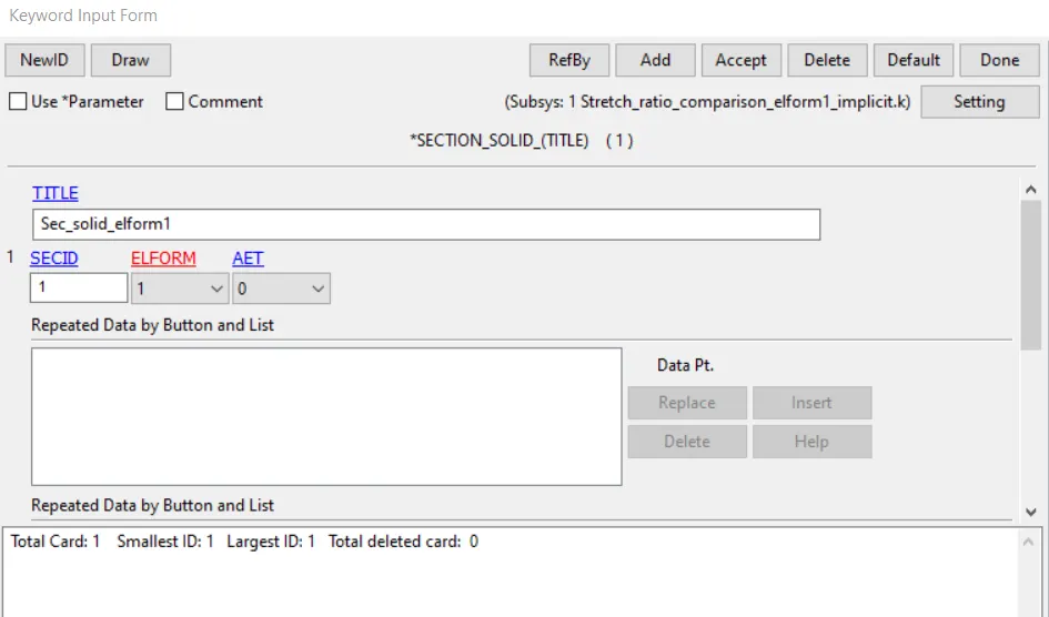
Figure.2.*SECTION_SOLID card
- Define a *MAT_OGDEN_RUBBER card and fill in the details given in the reference Material model provided. Now assign this material card to the created box.
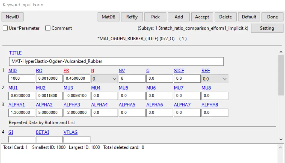
Figure.3.The material card
- Open LSPP. Create a box using solid Hexa elements as such that the dimensions are 10*10*10 with 10 elements in each direction. This can be done using the Shape mesher option under the Mesh panel.
- Creating boundary conditions
- We need to perform a tensile test on the box. Therefore, we have to fix one end of the box and impose some displacement on the other end.
- For fixing one end, we will use the *BOUNDARY_SPC_SET card. Note: All the nodes on the fixed face must not have any rotational DOF and they should be restricted from moving along the x-axis. The row of nodes along the center of the face should be restricted to move laterally. Thus we will create 3 cards for fixing this face.
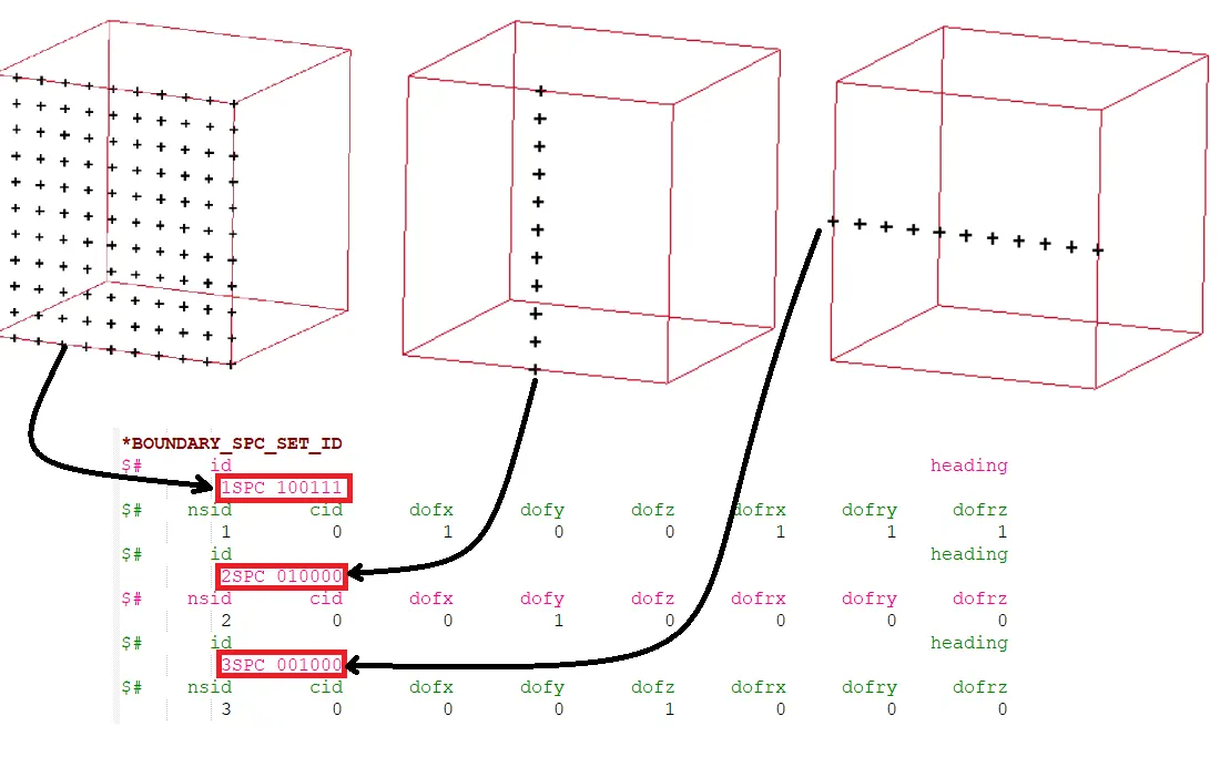
Figure.4.The boundary conditions for fixing one face of the cube
- For imposing a displacement, we will use the *BOUNDARY_PRESCRIBED_MOTION_SET card. Note: We need to plot graphs up to a stretch ratio of 5. Thus, we need to make sure that the displacement given at the moving face is large enough for getting a stretch ratio of 5. We can find the minimum displacement required for a value of 5 as follows: Stretch ratio, `lambda=1+epsilon_e` , where `epsilon_e` is the Engineering strain`=(deltal)/l`.Therefore, we need to find the value of `deltal` for which the Stretch ratio, `lamda=5``=>5=1+(deltal)/10=>deltal=40mm`. Thus we will define a displacement curve such that a displacement of 50mm is imposed on the moving face.
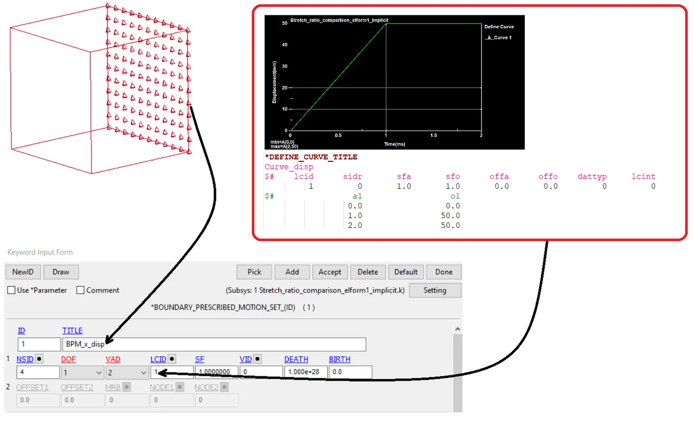
Figure.5.The Boundary Prescribed Motion card for imposing displacement in the x-axis
- Setting up the control cards for implicit analysis
- Create a *CONTROL_IMPLICIT_GENERAL card and put IMFLAG = 1 for running the analysis implicitly. Set DT0 = 0.01
- Create a *CONTROL_IMPLICIT_AUTO card and put IAUTO = 1. This will make LS Dyna automatically adjust time step, so that the time step values are between the DTMIN and DTMAX values such that the solver tries to maintain the number of iterations for achieving convergence, within the band defined by the ITEOPT and ITEWIN values.
- Create a *CONTROL_TERMINATION card and set the end time as 1. Note: In an implicit analysis, time is not really time. So here, the first time step will be 0.01(as defined in the *CONTROL_IMPLICIT_GENERAL card. Then the solver will see how many iterations is it taking for convergence and if that number is lying outside the band defined in the *CONTROL_IMPLICIT_AUTO card, it will adjust the time step in order to bring the number within the band. The run will terminate once 1 ms is reached.
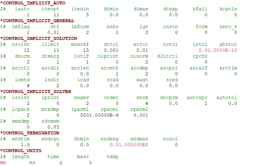
Figure.6.The Control cards created
- Making the output requests
- Request for d3plot using the *DATABASE_BINARY_D3PLOT card.
- Create a *DATABASE_EXTENT_BINARY card to record the strain and plastic strain tensors using the STRFLG = 011
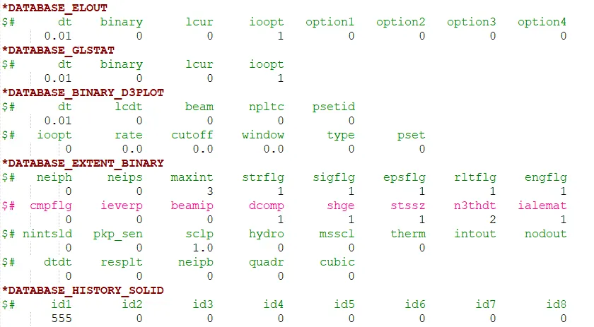
Figure.7.The output requests made
- Post-processing
- Run the analysis using the LS Run application(The use of control unit card throws an error when run using the launch manager but no such error on running the same keyword file using the LS RUn application. Not sure what the issue is.).
- Open the keyword file and the d3plot file in LSPP. Play the animation to visualize the results of the applied boundary conditions. Generate the stress and strain contour animations.
- Now we need to select one element and use the History option to plot the x-stress and x-strain for that element. In this case, I have selected element number 555 which is approximately at the center of the box. Save the plot details as an excel file. The stress and strain values recorded in LS Dyna are true stress-strain values. We are asked to plot the Engineering Stress vs stretch ratio for the four cases. We need to calculate the Engineering stress-strain values from the true stress-strain values taken from the LS Dyna plots as shown below:
We know, True stress, `bbsigma_(true)=bbsigma_(engg)*(1+bbepsilon_(engg))=>bbsigma_(engg)= bbsigma_(true)/(1+bbepsilon_(engg)`
Similarly, True strain, `bbepsilon_(true)= ln(1+bbepsilon_(engg))=>bbepsilon_(engg)= e^(bbepsilon_(true))-1`
- Using the above relation, calculate the Engineering stress-strain values and tabulate the results. Calculate the stretch ratio values as well. Stretch ratio, `bblamda = 1+bbepsilon_(engg)`.
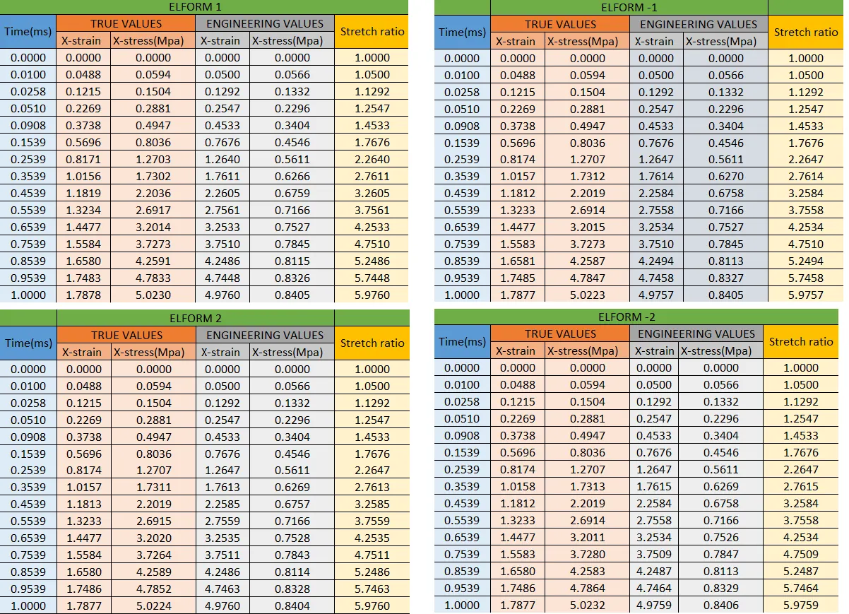
Figure.8.Calculations
- Plot the Engineering stress vs stretch ration curves for each of the four cases and compare the results.
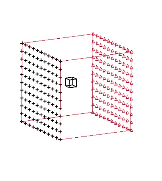
Figure.9.The element number 555, for which the stresses and strains have been plotted
RESULTS:
- Tension test stress-strain contour animations
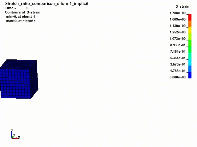
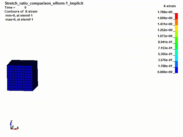
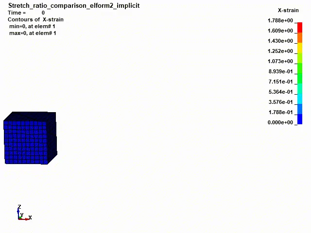
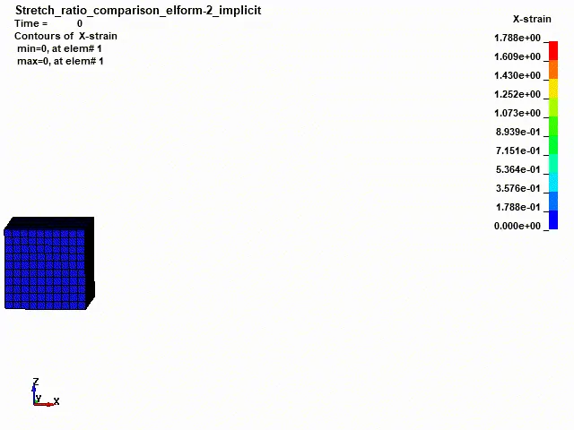
All the cases case identical contours for both stress and strain with not much to differentiate between them. Max stresses recorder are 5.023 MPa, 5.026 MPa, 5.023 MPa, and 5.024 MPa respectively for cases 1, 2, 3, and 4. Max strains recorded is 1.788 for all the cases.Cases Elform value Animation Stress_contour Strain_contour Case 1 1 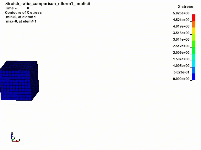
Case 2 -1 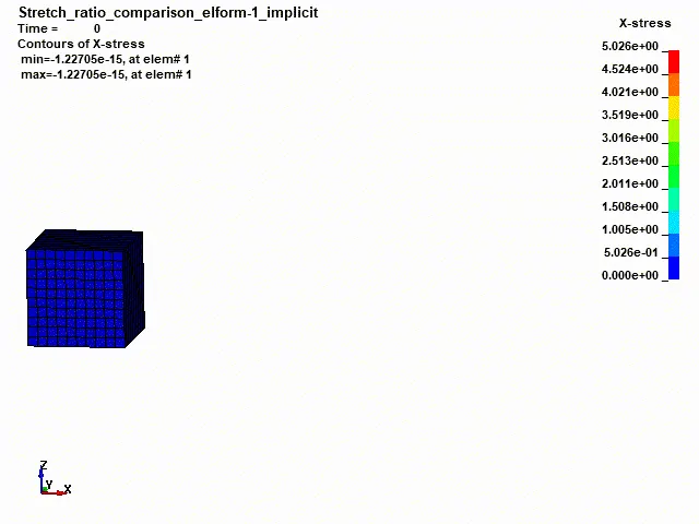
Case 3 2 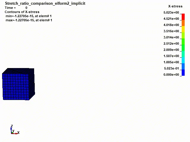
Case 4 -2 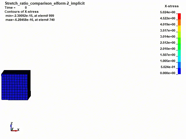
- Engineering stress vs stretch ration curves:
The curves for all the cases are nearly the same with the Engineering stress value recorded to be ~0.8 MPa for a stretch ratio of 5. On comparing the curves plotted with the original curve for the material model, we see that not much stress has been induced on the elements. The original curve shows stress of ~1.6 MPa corresponding to a stretch ratio of 5, whereas the plots we have generated only show ~0.8 MPa for the same stretch ratio. If we compare the shape of the original curve and the generated ones, we can also see that the shape of the curves is similar up to a stress of 0.8 MPa but the difference is that 0.8 MPa stress in the original curve corresponds to a stretch ratio of 2 compared to 5 in the generated curves. This difference could be due to the fact that we have not followed the tension test standards correctly. In a proper tension test, the specimen has to be of a particular size and everything is standardized. In our case, we have just used a random specimen and applied some arbitrary displacement. Thus the two results should not actually be compared.Cases Elform value Curves Case 1 1 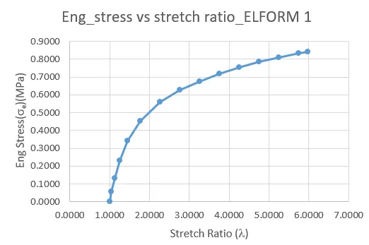
Case 2 -1 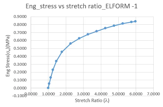
Case 3 2 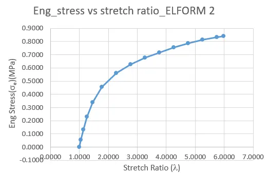
Case 4 -2 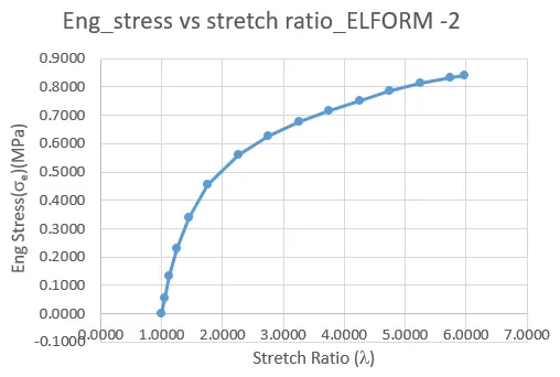
The actual stress vs stretch ratio curve for Ogden material
- Engineering stress vs stretch ration curves:
CONCLUSIONS:
- The tension test was simulated for a cubical box modeled with Hexa elements and Hyperelastic Ogden material model. The test was performed with elforms 1, -1, 2, and -2.
- The true stress and strain values were used to calculate the engineering stress and strain values.
- The stretch ratio was calculated for all the cases and a plot of Engineering stress vs stretch ratio curves were created and compared.
- An implicit method was used to solve this tension problem as the rate of displacement imposed on the model was very low and thus, it was similar to a quasi-static analysis on a hyperelastic elastic non-linear material. An explicit method can also be employed in solving the same problem but it will take more time for the solver to solve it explicitly.
Click here to view the completed files.