Comparing the event of a rail crashing on to a rigid wall using default shell element properties and recommended shell element properties in Radioss.

Objective:

1. To simulate the event of a rail crashing on to a rigid wall using both the default and the recommended shell element properties and to compare the two results.

Procedure:

1. CASE 1: Simulation with default shell element properties
   1. Import the given radioss starter file into Hypermesh using import>>solver deck>> Filename_0000.RAD. Fig 1. The imported solver deck file
   2. Change the run time to 55 ms by editing the ENGINE_RUN card. This card will decide how long the simulation has to run. Fig 2. The ENGINE_RUN card Fig 3. The radioss engine file showing the new run time
   3. One of the objectives is to change the number of animation steps to between 25 and 60. The number of animation files generated will be decided by the Time-frequency entered in the ENG_ANIM_DT card. Thus we need to edit the card value. We are keeping the Tfreq value as 1 so that we get 55 animations generated during the total run time of 55 ms. Fig 4. The ENG_ANIM_DT card Fig 5. The radioss engine file showing the Tfreq value
   4. Note that the properties of the shell elements have been kept as default. This can be checked by looking in the Property cards. Fig 6. Hat-section property Fig 7. Close-out-panel property
   5. We want to extract the values of Internal energy, Von misses stress and Hourglass energy throughout the simulation so that we can plot them in a graph or create a contour animation. This is done by checking the respective boxes under the ENG_ANIM_ELEM card. We also require to record the displacements and velocities. This is done by checking the respective boxes under the ENG_ANIM_VECT card. The Output blocks created also decides the outputs requested by the Engine input file. Fig 8. ENG_ANIM_ELEM card Fig 9. ENG_ANIM_VECT card
   6. Export the edited solver deck by using the Export >>Solver deck option. On exporting, Hypermesh will create two .rad files in the target location. The file formated as filename_0000.rad is called the starter input file and the one formated as filename_0001.rad is called the engine input file. The starter input file contains the model definition. The Starter diagnosis possible errors in the models and outputs a binary restart file. The Engine executes the actual computation. It expects the binary file produced by the Starter plus a Runname_run#.rad input file in Radioss. The Engine Input file describes the case-control. The Engine produces output files for animation, plotting (time history), and restart. Fig 10(a). Exporting the solver deck Fig 10(b). Exporting the solver deck
   7. Now we need to run the analysis in Radioss. Go to the Radioss panel in the Analysis menu of Hypermesh and load the Starter input file from the target folder and hit the Radioss button. This will run the simulation and generate the animation file in .h3d format and the time history file as runname_T01. The Time history file contains all the values of the requested outputs recorder based on the value of time_frequency defined in the ENG_TFILE card. Fig 11(a). Running the analysis in Radioss Fig 11(b). Running the analysis in Radioss
   8. On running the Analysis, a Hyperworks solver window will open. On the completion of the run, we can view the engine output file by clicking on the output option in the drop-down at the bottom right corner of the Hyperworks solver window or by opening the runname_0001.out file in a notepad by going to the target folder. Fig 12. Opening the Engine output file from the Solver window
   9. In the engine out File, we need to check if the energy errors and mass errors are within the limit. The accepted value of energy errors is between 5% to -15% and mass error is 2-3 %. In this particular case, we can see the energy error generated during the run is -10.3% which is acceptable. The mass error is recorded as 0.016% which is also within the limit. Since the energy errors are within the acceptable range, we can now move on to inspect the animation generated and plot the required graphs for post-processing. Fig 13. Energy error check
   10. To view the animation file, we can either use the Result option in the Hyperworks solver window or import the .h3d file in Hyperview. Fig 14. Opening the .h3d file from the Solver window
   11. Play the animation to see the whole simulation. Note that the animation will be recorded based on the start time entered in the ENG_ANIM_DT card. The animation looks a bit unrealistic. We will further analyze the result by viewing different contours and plotting various output data against the run time. Fig 15. Rail crash simulation
   12. Lets now generate the displacement, velocity, and von-misses stress contour plots for the simulation. Fig 16. Switching to contours in Hyperview Fig 17. The Displacement contour Fig 18. The Velocity contour Fig 19. The Von-mises stress contour
   13. Now, let us generate the necessary plots. Open a new page and switch to Hypergraph 2D. Load the time history file from the target folder. Fig 20(a). Opening the time history file in HyperGraph 2D Fig 20(b). Opening the time history file in HyperGraph 2D Fig 20(c). Opening the time history file in HyperGraph 2D
   14. Now that the runname_T01 file is loaded, we can choose the Y-AXIS parameters as needed and generate the plots for Internal Energy, Contact Energy, Total energy, and Hourglass energy vs time. Also generate the plots for Rigid wall forces and time step. Note that the units for recorded values are based on the Units selected in the Starter input file. In our case, Lenght is in mm, time is in ms and mass is in g. Fig 21. Time vs IE_KE_CE_HGE_TE Fig 22. Time vs Rigid wall forces(Normal and tangential) Fig 23. Time vs Rigid wall forces(Resultant) Fig 24. Time vs Timestep
   15. Now, all the requested contours and plots have been generated. To view the output files, click here
2. Case 2: Simulation with recommended shell element properties
   1. Import the given radioss starter file into Hypermesh using import>>solver deck>> Filename_0000.RAD.
   2. Repeat steps (i - iii) from Case 1.
   3. We have to now change the shell element properties to their recommended values for an explicit crash. Fig 25. Hat-section property Fig 26. Close-out-panel property
   4. Repeat steps (v - viii) from Case 1.
   5. In the engine out File, we need to check if the energy errors and mass errors are within the limit. The accepted value of energy errors is between 5% to -15% and mass error is 2-3 %. In this particular case, we can see the energy error generated during the run is -0.1% which is excellent. The mass error is recorded as 0.016% which is also within the limit. Since the energy errors are within the acceptable range, we can now move on to inspect the animation generated and plot the required graphs for post-processing. Fig 27. Energy error check
   6. To view the animation file, we can either use the Result option in the Hyperworks solver window or import the .h3d file in Hyperview. Fig 28. Opening the .h3d file from the Solver window
   7. Play the animation to see the whole simulation. Note that the animation will be recorded based on the start time entered in the ENG_ANIM_DT card. The animation looks a bit unrealistic. We will further analyze the result by viewing different contours and plotting various output data against the run time. Fig 29. Rail crash simulation
   8. Lets now generate the displacement, velocity, and von-misses stress contour plots for the simulation. Fig 30. Switching to contours in Hyperview Fig 31. The Displacement contour Fig 32. The Velocity contour Fig 33. The Von-mises stress contour
   9. Repeat step (xiii) from Case 1.
   10. Now that the runname_T01 file is loaded, we can choose the Y-AXIS parameters as needed and generate the plots for Internal Energy, Contact Energy, Total energy, and Hourglass energy vs time. Also, generate the plots for Rigid wall forces and time step. Note that the units for recorded values are based on the Units selected in the Starter input file. In our case, Lenght is in mm, time is in ms and mass is in g. Fig 34. Time vs IE_KE_CE_HGE_TE Fig 35. Time vs Rigid wall forces(Normal and tangential) Fig 36. Time vs Rigid wall forces(Resultant) Fig 37. Time vs Timestep
   11. Now, all the requested contours and plots have been generated for Case 2 as well. To view the output files, click here.

Result Study:

Serial No.	Parameter
1	Crash animation
	Case 1	Case 2
	The case 1 simulation seems totally unrealistic with extensive amount of deformations in elements even at the opposite end of impact region. Whereas the case 2 simulation is more realistic with the opposite end of the rail remaining intact until the last part of the animation. This difference could be due to some of the elements in case 1 simulation moving into Hourglass mode. As the shell formulation with Ishell = 24 (QEPH) was used for case 2, the hourglass mode seems to be successfully prevented.
2	Displacement contour
	Case 1	Case 2
	In both the cases, Node no.169 experienced the max deformation and the magnitude remained nearly similar with the displacement being slightly higher in Case 2. The Node no.716 is the one coming in contact with the rigid wall and it remains at the same position throughout the simulation. Hence it is the node with the least displacement.
3	Velocity contour
	Case 1	Case 2
	Initially, the velocity is nearly 15 -16 m/s throughout the rail except the region impacting the rigid wall. As the simulation runs, the velocity is getting decreased for nodes getting closer to the rigid wall.
4	Von-mises stress contour
	Case 1	Case 2
	The von-mises stresses can be clearly seen to increase at the bending regions in Case 2 which is not clearly visible in Case simulation. This can be due to the absence of hourglass energy in Case 2. Maximum von-mises stress are noted as 349.9 Mpa and 349.1 Mpa in case 1 and 2 respectively.
5	Time vs Energy plots
	Case 1	Case 2
	The effect of the recommended shell properties can be clearly observed in the Energy plots. The choice of Ishell = 24(QEPH) has reduced the hourglass energy to zero in Case 2. In Case 1, it can be seen that the Hourglass energy is increasing with Run time. Contact energy remained null in both cases. The kinetic energy can be seen to have decreased during the simulation due to the impact. However, this decrease in kinetic energy is actually due to its conversion into Internal energy or potential energy due to the collision. The decrease in Total energy in case 1 is against the laws of physics. The elimination of Hourglass energy has resulted in the total energy remaining constant throughout the run time in Case 2, thus removing this error. Note that the energy error got decreased from -10.3% in case 1 to just 0.1% in case 2.
6	Time vs Resultant rigid wall forces plot
	Case 1	Case 2
	The resultant force is maximum at the start of the run when the rail has started to crash against the rigid wall. The force then decreases due to the deformation of the elements at the regions which got bent during the run. The spikes in the plot depict the instances at which new elements are impacting against the rigid wall. In case 2, the forces can be seen to have reduced to nearly 0 N at ~7ms. This is unrealistic. In Case 2, this error has been removed due to the modified shell properties. The peak towards the end of the plot in Case 2 is due to many new elements impacting the rigid wall at ~53ms. This is evident from the displacement contour as well.
7	Time vs Timestep plot
	Case 1	Case 2
	The Timestep in Case 1 can be seen to have reduced significantly during the run. In case 2, the increase in stiffness due to the choice of Ishell = 24(QEPH) for preventing the Hourglass modes must have increased the timestep during the run. The minimum timestep for case 2 is ~0.00183ms whereas the same for case 1 is ~0.17ms.

Conclusion:

1. The use of recommended Shell element properties has resulted in a more realistic and physically acceptable simulation.
2. The most significant change observed was the elimination of the Hourglass modes.
3. The maximum Von-mises stress was noted to be 349.9 Mpa in Case 1 and 349.1 Mpa in Case 2.

Hourglass energy:

Hourglass modes are element distortions that have zero strain energy. The 4 node shell element has 12 translational modes, 3 rigid body modes, 6 deformation modes, and 3 hourglass modes. As the distortions in the hourglass modes are not leading to any strain energy, it makes the whole system unstable. Thus Hourglass modes need to be avoided. Hourglass is observed in coarse meshes and shell formulations with under-integration or elements with only a single integration point at the center. In such cases, sometimes, the effect of displacement of nodes might not get reflected in the strain calculated at the single integration point. Thua this will lead to distortions with no resulting strain energy. Hourglass is not present in 3 noded tria elements and tetra elements.

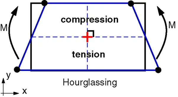Fig 38. Hourglass effect on a quad element

In the figure, it can be seen that even though the nodes have displaced at both ends, the length measured along the dotted line in the X-axis is not changing. Thus if we assume the center point to be the integration point, the effect of the displacements of the nodes has not been reflected on the measurements at the integration point.

There are two methods to remove Hourglass:

1. Viscous method / Perturbation method:
   • The hourglass deformation is detected with the relative motion (velocity) of the nodes.
   • When hour glassing is detected, a force is applied on the node to stabilize the deformation.
   • This force is defined according to the element stiffness (Young modulus, yield stress, plastic tangent..)
   • This force introduces artificial energy (named hourglass energy). The more the hourglass energy, higher will be the chances of instability. This method is used in Ishell= 4(Q4) shell element formulation.
2. Physical method / Stiffness method:
   • In the physical method. the solver increases the stiffness of all the elements to avoid the occurrence of hourglass modes. This is the most efficient method of Hourglass removal.

1. • The Ishell =24(QEPH) shell element formulation uses this method to prevent hour glassing. This shell element formulation is the optimum for accuracy and cost.

Click here to view the Completed files.