Week 5 - Turbulence modelling challenge
Turbulent flows are characterised by a large range of vortical structures at different scales, both in time and space, which interact with each other and exchange energy. The largest scales contain most of the kinetic energy for the flow. As larger structures are broken into smaller ones, this energy is transferred to progressively smaller scales. The process of energy transfer from large to small scale is called direct energy cascade and it continues until the viscous dissipation can convert the kinetic energy into thermal energy. The scale at which this occurs is referred to as Kolmogorov length scale, after the mathematician Andrey Kolmogorov who worked on the energy cascade in turbulence.
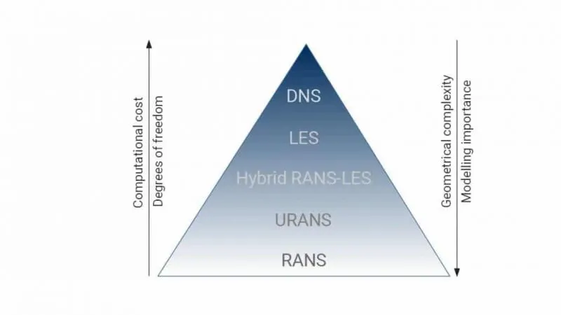
RANS & URANS
Turbulence models aim to represent the effect of turbulence via the closure of unknown Reynolds stress terms. Turbulence models are generally classified based on the number of additional equations that are required in order to model the effect of turbulent on the flow. Models range from very simple algebraic relations and increase in fidelity and complexity as the number of equations used is increased. RANS modelling is the most common and widespread approach in industrial applications. If the flow of interest is characterised by moving parts or periodic flow feature, these can be resolved using unsteady RANS (URANS).
An averaging operation can be applied to the Navier-Stokes equations to obtain the mean equations of fluid flows called Reynolds Averaged Navier-Stokes (RANS) equations. These are very similar to the original equations but contains some additional terms in the momentum equations called Reynolds stress terms that are unknown and need to be modelled.
All RANS models have some limitations due to the modelling assumptions used to derive the mathematical formulation of the model. For certain applications, it might be required to use more detailed approaches that instead of modelling all of the turbulence scales, try to resolve the most energy containing structures of the flow. This approach is called Large Eddy Simulations (LES).
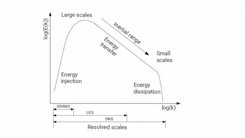
Large Eddy Simulations (LES).
In LES, the smallest scales of turbulence are spatially filtered out while the largest, most energy containing scales are resolved directly.
Due to the nature of turbulence, at a very small scale, the flow structures tend to be similar to each other even in different applications. This allows the use of simpler turbulence models that tend to be more universal and can be applied to several applications with a reduced requirement of model tuning.
Similarly to RANS modelling, in LES turbulence models aim at resolving the unknown terms in the filtered Navier-Stokes equations, called the Sub-grid Scale stresses. The term comes from the fact that in most LES models, the filtering of the equations is obtained at mesh size level, relegating the modelling to flow scales smaller than the grid size.
LES modelling offers increased range of applicability and increased fidelity of the solution but all of this comes with an increased computational cost due to the time step requirements, as we can no longer consider the flow steady, and increased mesh resolution required to capture more details of the flow.
There is a family of turbulence models where the benefits of LES modelling are being exploited while retaining the efficiency of RANS models where LES would be too expensive. These go under the name of hybrid RANS-LES models.
The majority of the mesh resolution tends to be in proximity of surfaces and bodies of interest as in LES the flow needs to be fully resolved near the wall. The cost of LES can therefore be greatly reduced if the constraints of the increased resolution near the wall can be relaxed. One of the most common hybrid approaches uses LES modelling away from the walls and RANS modelling near the wall. This approach is called Detached Eddy Simulation (DES). The DES approach is becoming very popular in industrial applications as it helps overcoming some of the limitations of the RANS models as well as offering increased insight in the solution as the simulation is always run as unsteady flow, even for cases that have a steady state solution, and the finer spatial resolution allows to study detailed behaviour of the flow of interest. All of it at a reduced cost compared to a fully fledged LES approach.
Direct numerical simulation (DNS)
A direct numerical simulation (DNS) is a simulation in computational fluid dynamics in which the Navier-Stokes equation are numerically solved without any turbulence model.This means that the whole range of spatial and temporal scales of the turbulence must be resolved. All the spatial scales of the turbulence must be resolved in the computational mesh, from the smallest dissipative scales (Kolmogorov scales), up to the integral scale L, associated with the motions containing most of the kinetic energy.
Procedure
a.The file was copied as it is into spaceclaim.
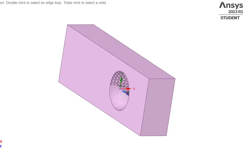
b.The was then meshed with an element size of 0.2mm
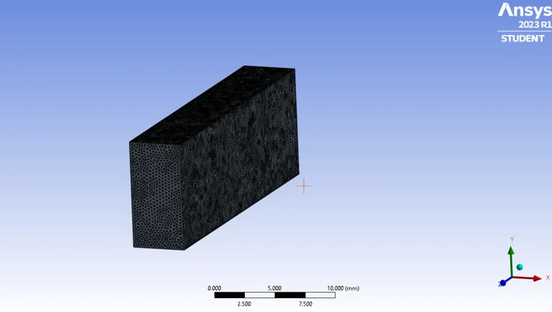
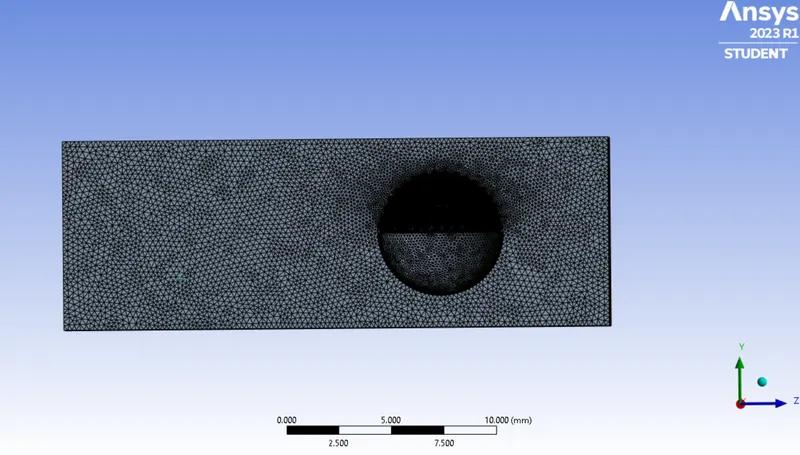
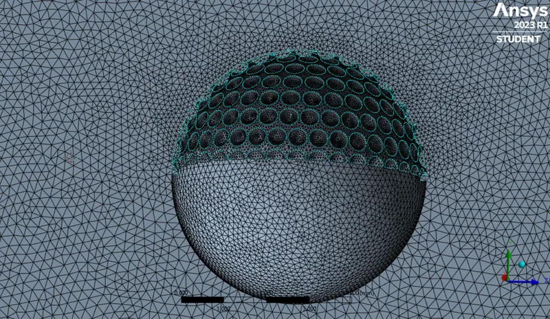
Nodes = 738063
Elements = 507935
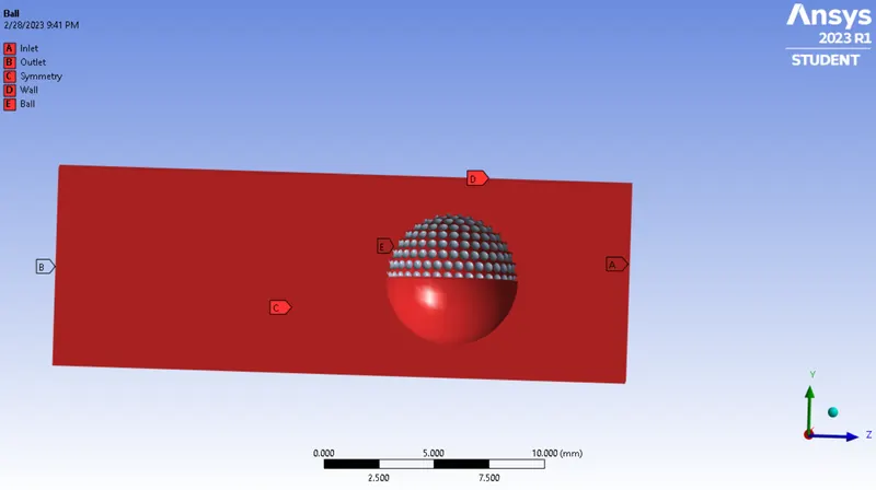
c.The appropriate naming selections were given.
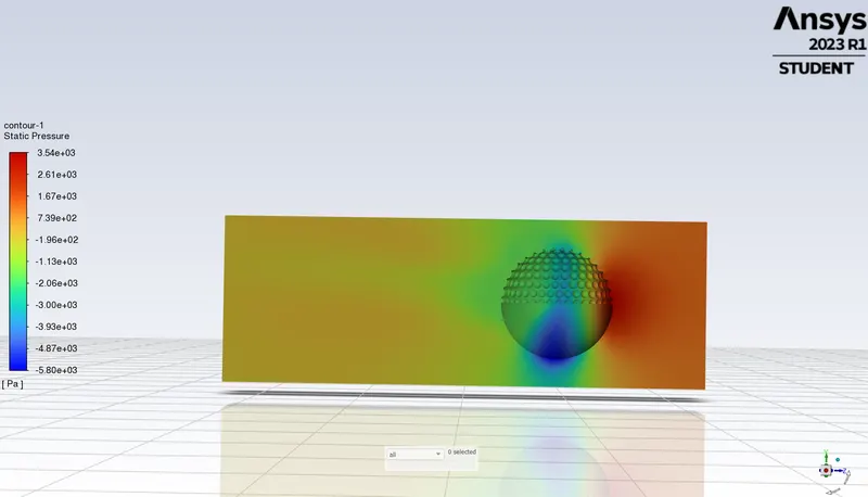
d.The velocity given here is 60 m/s.
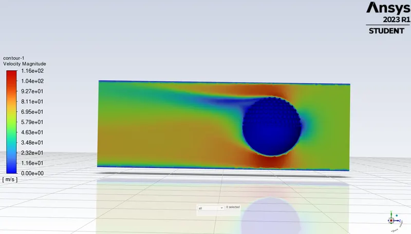
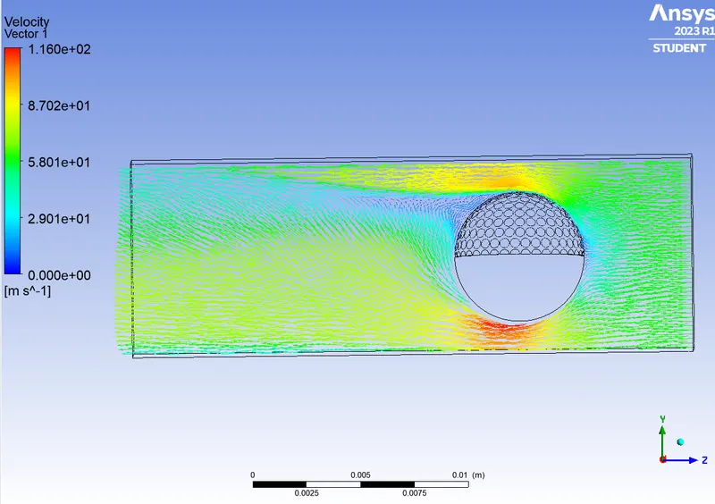
From the above figure we can see that the recirculation region is behind the ball and we can see that velocity is low on the uneven surface of the ball compared to the smooth surface which causes a wake region to be formed on the ball (which has very velocity formed in that area) due to this the ball will move in the downward direction.
Result
The required literature survey has been done on various turbulence models .A 3-D simulation was performed on a golf ball and the reciculation region was explained.