Week 5 - Turbulence modelling challenge

Aim

Perform a literature review on the various turbulence models and conduct a flow simulation over the given golf ball at a velocity of 60m/s and explain the recirculation region, further estimate the direction the ball will curve based on the visualization of the wake region.

Introduction

Turbulent flow is characterized by its highly random and stochastic nature. Unlike laminar flow, turbulence is expensive to resolve and often requires a modeled approach using various assumptions. The mathematical models used to predict these turbulent phenomena are called turbulence models and can be classified based on their modeling approach.

1. RANS
2. LES
3. DNS

1. RANS (Reynolds Averaged Navier Stokes)

RANS-based turbulence models involve the time averaging of the Navier-Stokes equations upon which a Reynolds Decomposition is conducted which splits the properties into mean and fluctuating terms as seen below.

`phi = bar phi + phi'`

Upon substituting this formulation to the continuity and momentum equations, a matrix can be generated with all the fluctuating velocities in the flow as shown below (2-dimensional)

`rho [[bar (u'u'), bar (u'v')],[bar (v'u'),bar (v'v')]]`

The terms in the above matrix are often termed the Reynolds stresses and the matrix is called the Reynolds stress tensor. The objective of the RANS Models is to evaluate these Reynold stresses using closure models.

One such closure model using the Boussinesq Hypothesis is the Eddy viscosity model, which introduces the eddy viscosity term as a constant of proportionality relating the turbulent stresses to the mean velocity gradients. With this relation, the system of equations will have no more fluctuating terms and therefore makes computing less expensive and quicker.

Finding the eddy viscosity term in the flow can be done by multiple methods and each varies case by case based on the type of flow. Some of the methods are:

Zero Equation Model

An example of this model is the Mixing length model which involves the use of a direct analytical relation to estimate the eddy viscosity. This model fails to account for the transient behavior of eddy viscosity and hence its usage is highly specific.

One Equation model

The Spalart-Allmaras model is a good example of the one equation model where the turbulent eddy viscosity is estimated directly using one PDE. This model is suitable for attached flows particularly used in external aerodynamics,

Two Equation models

There are multiple two-equation models like the k-Epsilon, the K-Omega models and their respective variants. These involve the estimation of the turbulent kinetic energy in the flow and a second property which is the rate of dissipation of kinetic energy either in the formulation of `epsilon` in the K-Epsilon model or `omega` in the k-Omega models.

Second Order Models

This method involves the usage of individual transport equations for each of the Reynolds stresses. This method is often expensive and requires a larger computational budget compared to the other RANS models but is also the most accurate.

2. LES (Large Eddy Simulations)

This model involves the direct numerical resolution of the Navier-Stokes equations on the larger eddies in the flow. The sizings of the eddies are based on the Kolmogorov scale. The LES models capture at least 85% of the turbulent kinetic energy in the flow which is often in regions of larger eddies. The smaller eddies are then modeled using the subgrid models similar to RANS formulations.

3. DNS (Direct Numerical Solution)

The DNS model performs a complete Navier-Stokes resolution on all the eddy scales in the flow making it the most expensive and highest accuracy solver currently available. This method is currently only used in advanced research involving small 3D sections or 2D profiles.

According to the Kolmorgorov scale,

`eta propto (1/(Re^(3/4)))`

If each dimension in the 3D volume mesh is required to be below the kolmorgorov scale then,

Volume of each cell ` propto (1/(Re^(9/4)))`

Which then implies,

No of cells` propto (Re^(9/4))`

This gives rise to an absurdly large number of cells, especially in the case of external aerodynamic turbulence where Reynolds number may be in the millions leading to a cell count requirement of about `(100000)^(9/4)` which takes the effective cell count to the billions. Hence, this model isn't feasible for industry applications yet.

Method

Geometry and Mesh

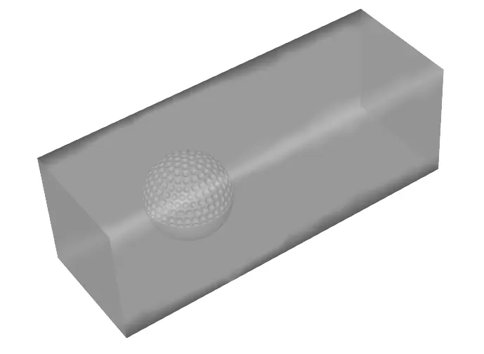
The given golf ball geometry and domain can be seen in the image below.

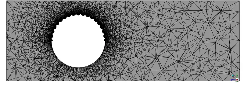
The mesh was generated using 2e-4m sizings on the face of the golf ball and provided with 6 inflation layers pertaining to a transition ratio of 0.6 to the bulk mesh. The resulting mesh has a cell count of 500k and can be seen below.

CFD Setup

The flow simulation was conducted on ANSYS Fluent 2022R2. Air was used as the fluid with default properties. The velocity at the inlet was set to a constant 60m/s with a pressure outlet downstream of the golf ball. All walls were set to no-slip conditions with a symmetry condition enabled on all other sides of the domain.

The steady-state pressure-based PV coupled solver was used to discretize the flow parameters. Turbulence in the flow was predicted using the two-equation K-Omega SST model. The second-order scheme was used to estimate the pressure, the second-order upwind scheme was used to estimate momentum, energy, and turbulence parameters. The solution was initialized by a standard initialization followed by and FMG initialization to quicken convergence. The simulation was run with pseudo transient time stepping with an automatic global conservative length scale. Convergence was checked by scaled residuals achieving 1e-4 units. The simulation converged within 150 iterations.

Results

The image below shows the recirculation region behind the golf ball plotted using velocity vectors.

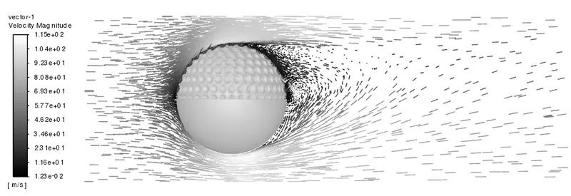
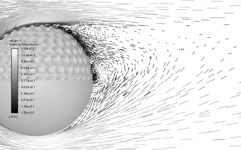
Flow separation can be observed behind the golf ball which leads to a suction that causes all the flow to be sucked behind it creating the recirculation seen in the images above. The velocity vectors show that the recirculation region has much lower velocity compared to the free stream.

The images below show the total pressure coefficient and the velocity of the flow field which can be used to identify the wake behind the golf ball.

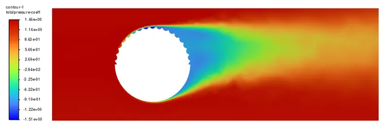
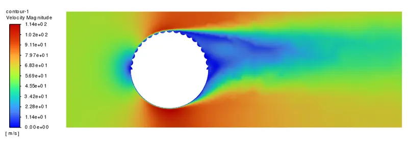
From the wake formation, it can be observed that a larger region of faster flow is present on the bottom surface of the golf ball. This fast-flowing flow will cause a reduction in pressure in the flow relative to the upper surface. This difference in pressure will push the ball downwards and hence the ball will have a curved tendency downwards.

The below image shows the evaluation of normal force on the ball in the vertical direction which shows a net downward force affirming the claim made from the wake observation.

Conclusion

A detailed literature study of the various turbulence models was performed followed by the flow simulation over the given golf ball. The simulation was conducted with a flow velocity of 60m/s. The recirculation behind the ball was observed using velocity vectors. Further, the wake behind the ball was analyzed and predicted that the ball will curve downwards. This claim was also backed by force estimation on the golf ball.