Turbulence modelling challenge

Turbluence is the one of the biggest mystery known to human kind. Because of its randomness, it is part one of those unsolvable million dollar phenomenon club. Luckily, even this randomness is not completely random, it does have some patterns. These patterns are none other than eddies.

Trubluence models have been created to solve for these eddies.

There are 3 Major types of Turbluence models.

1. DNS - Direct Numerical Simulations

2. LES - Large Eddy Simulation

3. RANS - Reynolds Averaged Navier Stokes

1. DNS

Direct Numerical Simulation, shortly known as DNS solves for even the smallest eddies. It does not use any modelling for that. This requires a very fine grid to capture the smallest eddies. This makes DNS extremly time consuming and computationally expensive.

According to kolmogrov's scale, the size of smaller eddies is inversely proportional to 3/4 th power of Reynolds number.

In 3-Dimensional terms, this makes the volume of element inversly proportional to 9/4 powers of Reynold number.

That means the total number of elements required to capture the smallest eddies would be directly proportional to 9/4th power of Reynolds number. This makes the Mesh very very finer and computationally expensive.

Hence, DNS is not suitable in most of the appliations. It is absurbdly expensive and time consuming.

2. LES

Large Eddy simulation, as the name suggests solves for only the larger eddies and neglects the smaller once.

Eddies in LES are resolved using Mesh. The mesh can resolve only those eddies that are smaller than width of two cells, these is because velocity is stored at cell centroids. It requires further modelling to take into account the effect of the smaller eddies. One such modelling approach is sub-grid modelling.

This means that the mesh sets the limitation for the minimum eddy size that can be resolved.

A high/good quality mesh resolves atleast 80% of the eddies. But how do we decide the correct mesh size.

To know the appropriate mesh size, we have to first run a RANS (discussed later) simulation. From the RANS simulation we obtain the value of the Integral Length Scale. The Mesh length must be atleast 5 times smaller than the integral length scale.

The integral length scale is the representative of all the eddies at that location. It is the length of an eddy at the average kinetic energy of all eddies. The integral length scale varies from location to location. Hence, the mesh also needs to be refined from place to place based on the requirement.

3. RANS

Velocity at every region in field can be splitted into Mean velocity componenet and fluctuating velocity component. Reynold averaging of the avier stokes equation gives rise to an additional term in the NS equation. This term contains the fluctuating component of the velocity. The term is named a sReynolds stress term.

The Reynolds stress term written interms of mean free velocity gives rise to a new unknown called as turbluent viscosity.

There are different approaches to calculate the turbluent viscosity term.

1. 1st order Models

Further classified into different models based on the number of PDE's used to solve for the turbluent viscosity term.

a. Zero Equation Models

b. One Equation Models

- Good for attached flows - Internal and External Aerodynamics

- Not good for flows with strong adverse gradients.

c. Two Equation Models

- k-Epsilon = solves for Turbluent Kinetic energy and Turbluent dissipation rate

Further divided into Standard, Realizable and RNG models

- k-Omega = solves for Turbluent Kinetic energy and Specific dissipation rate

Further divided into Standard and SST models.

2. 2nd order Models

Reynolds Stress models and Algebraic Stress models.

They are accurate, but expenisve.

They are sensitive to boundary conditions.

To know more about all the Turbluence models, check out "Fluid Mechanics 101" on Youtube.

Semi-Dimpled Golf Ball Simulation

1. Import the Geometry into Design Modeller.

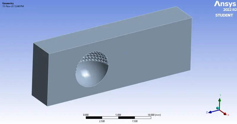
Since the geometry is symmetrical in nature, we can splice it as shown below.

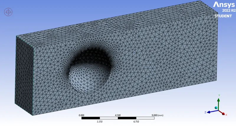
2. Meshing

3. Processing

Pressure based solver (Incompressible flow = Mach <0.3)

K-Omega SST (To capture phenomenon both close to and away frrom boundary layer)

Inlet - velocity based = 60m/s

Outlet - Pressure based = 0

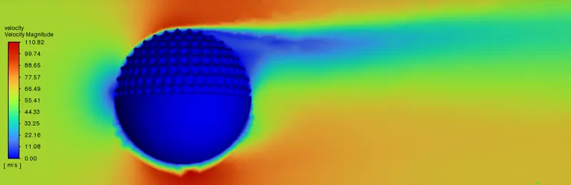
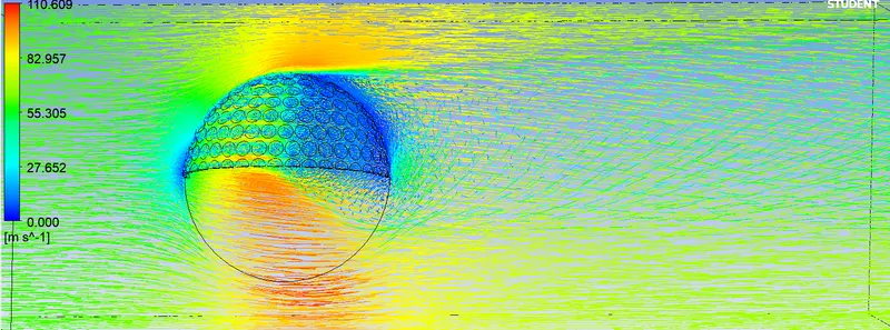
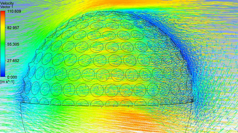
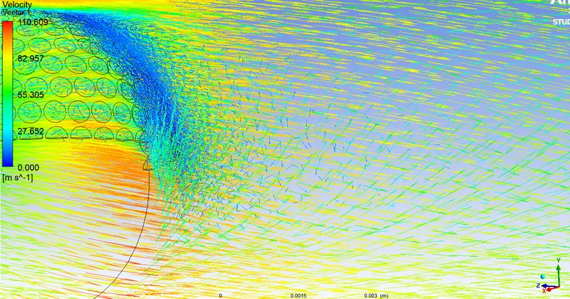
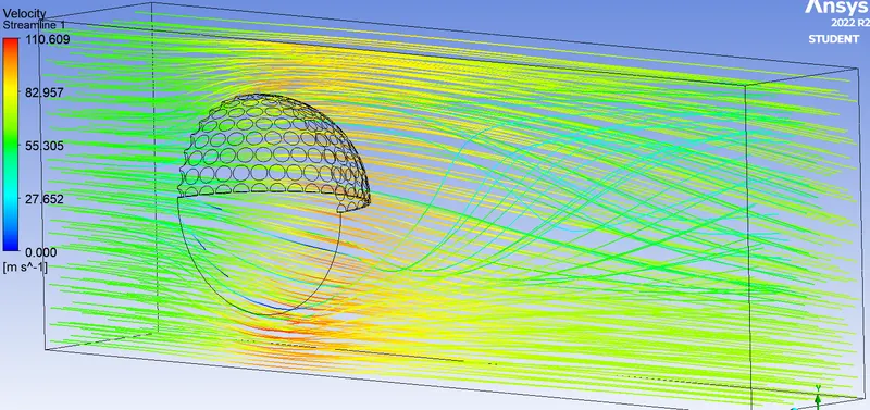
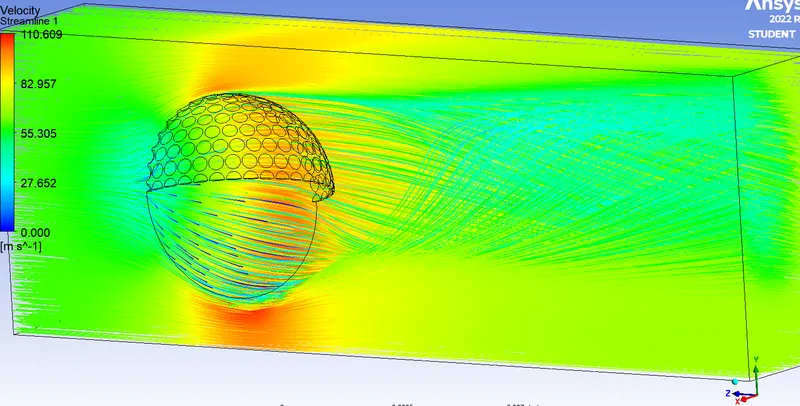
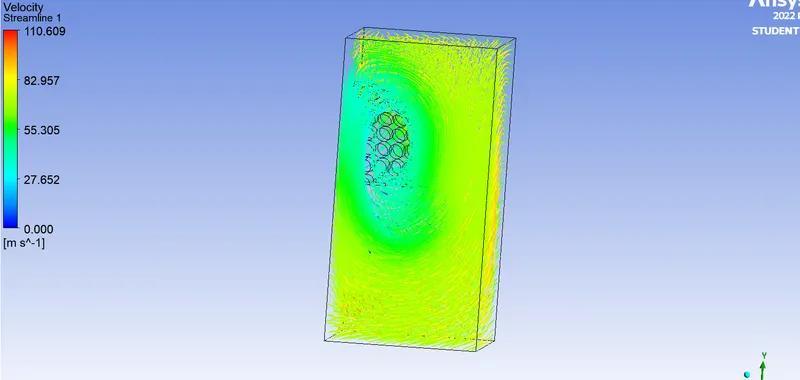
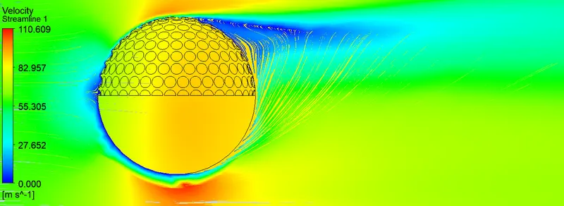
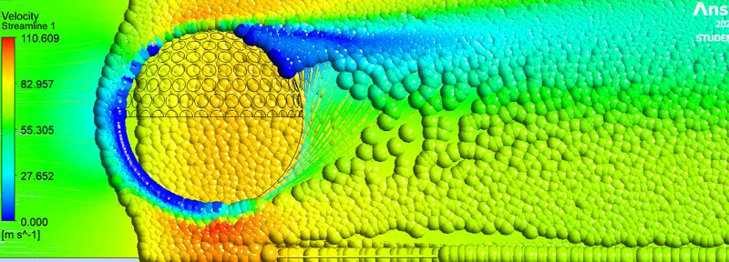
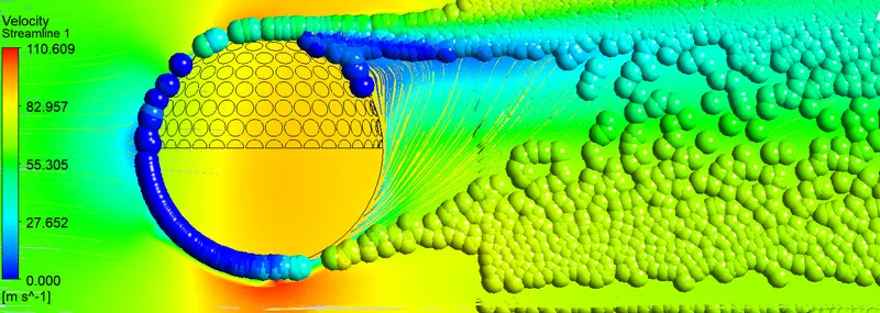
A low velocity region can be seen behind the dimpled part of the golf ball. This is because the flow stays attached for a long time due to the dimples and slows down considerably.

Conclusion

• High pressure infornt of the ball and low pressure behind the ball. This would create pressure drag.
• Behind the ball - High pressure region at the top and low pressre region in the lower portion.
  More pressure difference in the dimpled region = More Drag in the dimpled region = Torque = Spin
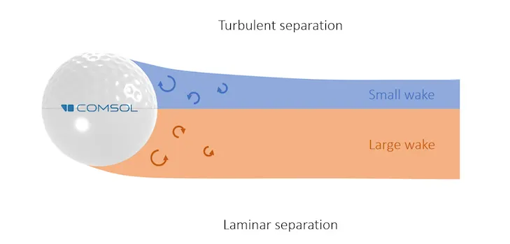
  Possible spin will be clockwise. (let me know in the comments section if my understanding about spin is correct)
• Delayed flow seperation in the top region due to dimples, see the video file attached.
• Since the flow is seperated earlier in the lower/smoother part, wake is preoduced early here.