Week 5 - Turbulence modelling challenge
Brief Overview of Turbulence models.
Flows can be classified as Laminar characterized by orderly flow, then transitional, and finally turbulent flow where the flow is highly unsteady.
For turbulent flows, the unsteadiness can be modeled by using Reynolds Averaging eg: u(t) = U+u' where U is the average value and u' is the fluctuating component.
The extra components of the RANS model are found by solving additional equations which are commonly referred to as turbulence models.
1. Mixing Length Model
They try to describe the stresses by using a simple algebraic formula for turbulent viscosity as a function of position.
2. 1 equation model - Spalart-Allmaras Model
The Spalart–Allmaras model is a one-equation model that solves a modeled transport equation for the kinematic eddy turbulent viscosity. The Spalart–Allmaras model was designed specifically for aerospace applications involving wall-bounded flows (Internal flows). specifically when the flow is attached to the body. The Spalart-Allmaras model has been implemented to use wall functions when the mesh resolution is not sufficiently fine.
3. 2 equation Models
K-e model
Here K is turbulent Kinetic Energy & e is the Turbulence dissipation rate.
Simplest turbulence model for which only initial & boundary conditions are not required
Most validated turbulence model
It is widely suited for confined flows
Standard K-e Model:
It uses the wall function for finding the values of turbulent kinetic energy.
Good for attached and turbulent flows
Realizable Model:
It goes for a modified equation for e.
Captures the physics more accurately compared to Standard Model
RNG Model:
Best suited for flows where swirl is present.
k-w Model:
Standard k-w model:
Used in Aerospace/turbomachinery industries
Good for flows with flow separation, recirculation.
SST K-w model
It uses a blender function allowing it to behave as a K-w model near the wall and as a K-e model away from the wall.
Wall Functions are mainly used to resolve the physics of the boundary layer.
It can be done either by using empirical relations or based on the wall grid distance (Y+).
Second-Order / 7 Equation Model
Algebraic Stress Model
It is mainly used for source-dominated flows, where convective and diffusive fluxes are negligible.
Reynolds Stress Model
These models use the exact Reynolds stress transport equation for their formulation. They account for the directional effects of the Reynolds stresses and the complex interactions in turbulent flows. Reynolds stress models offer significantly better accuracy than eddy-viscosity-based turbulence models while being computationally cheaper than Direct Numerical Simulations (DNS) and Large Eddy Simulations.
Reasons for DNS being not feasible for Kolmogorov scales.
Eddies refer to the swirling of the fluid when the flow regime is turbulent.
Large eddies will break into smaller eddies and sometimes small eddies combine to form large eddies which is called as energy cascading.
Large-eddy size `alpha (l/U_(infty))`
small-eddy-size `alpha(l/(Re)^(3/4))`
Kolmogorov's theory will describe how energy is transferred from larger to smaller eddies, and how much energy is contained in an eddy of a given size and how much energy is dissipated by an eddy of a given size.
Kolmogorov length scale `eta=((v)^3/(epsilon))^(1/4)` `eta=(U)^3/L`
Kolmogorov time scale `t_eta=(v/epsilon)^(1/2)`
Ratio of largest to smallest eddies
`L/eta=(L/mu^(3/4))*epsilon^(1/4)`
`L/eta=(L/mu^(3/4))*(U^(3/4)/L^(1/4))`
`L/eta=(L*U^(3/4))/(mu)`
`L/eta=(Re)^(3/4`
To model the eddies we have ensured that our grid size is able to capture/resolve the size of the eddies.
In DNS the equations are solved for a small scale `eta alpha (1/(Re)^(3/4))`
The grid size must be smaller than the length scale and for 3D it is applicable in all the 3 lengths
So for volume `alpha (1/(Re)^(9/4))`
the number of grid points necessary to resolve a turbulent flow in a numerical model is therefore proportional to `alpha Re^(9/4`
No of elements = `V/(DeltaV)`
Therefore the computational time and cost to run a 3D DNS simulation is high and therefore is used mainly for research purposes.
Golf Ball Simulation:
Case-Setup & Boundary Conditions.
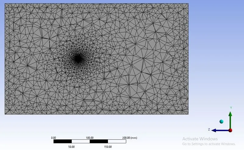
The given domain has meshed with an element size of 1.5 mm giving a total cell count of 4,47,667.
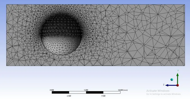
Pressure based steady solver is used here.
The k-w SST viscous model has been applied.
the working fluid is air at standard atmospheric conditions and the operating pressure is at 1 Atm.
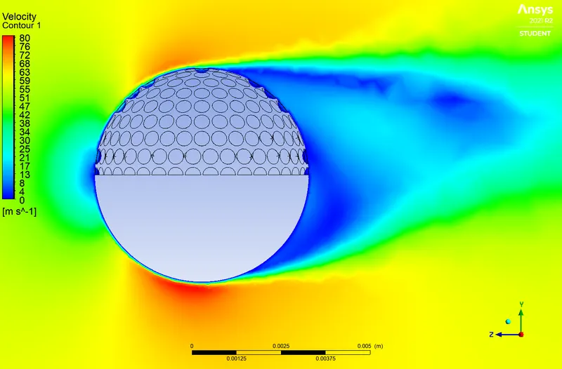
Velocity Inlet : 60 m/s
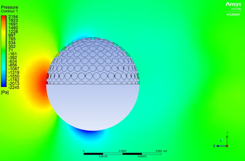
Pressure Outlet : 0 Pa (Gauge Pressure)
The cylinder surface is taken to wall BC with the no-slip condition for momentum.
Results
Pressure & Velocity Contours for the given domain.
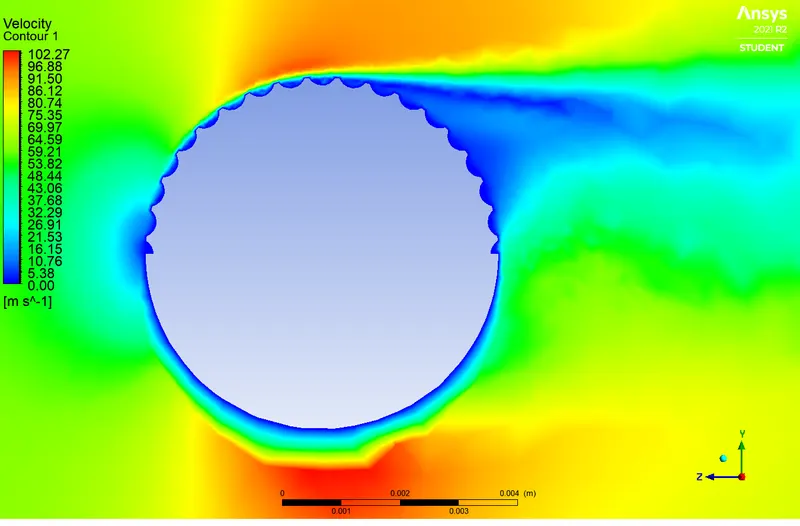
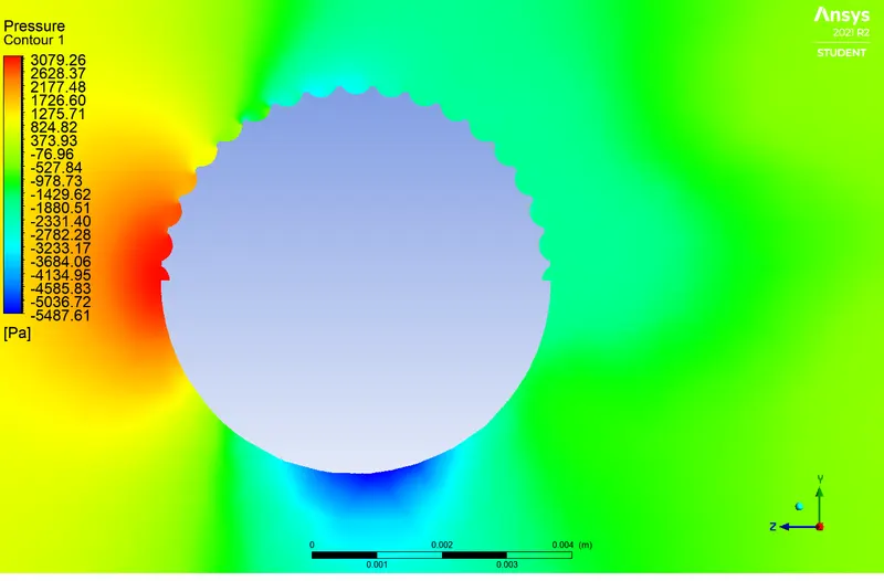
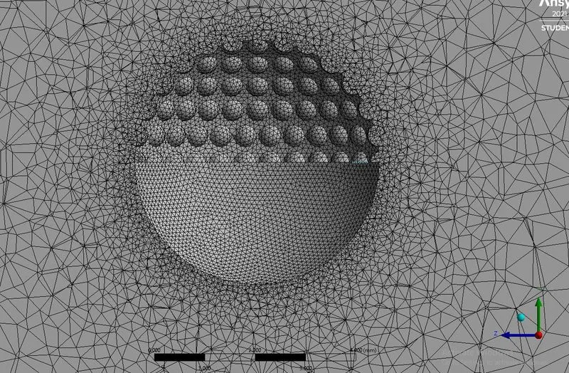
A second case was run with a larger domain and results obtained for the same are also presented below.
Mesh generated for the larger domain.
Conclusion:
Based on the contours we say that the ball will move down due to the low-pressure region at the bottom of the ball.